Wednesday Week 7: More hyperbolic spaces!

Introduction

Last class, wonderfully recounted by Michaela, we learned about hyperbolic groups and defined the terms quasi-isometry and quasi-isometric. Importantly, we showed that there is a quasi-isometry between any group and its Cayley graph, and that two Cayley graphs of the same group are always quasi-isometric. In today’s class we continued with a similar subject matter, focusing in on quasi-isometries. We will first present the theorem that quasi-isometries are equivalence classes on metric spaces with the motivation that quasi-isometries are able to preserve the hyperbolic structure of a group. Subsequently, we will define and discuss what it means to be $\delta$ -slim, showing several neat examples through figures.

We begin with a definition which was given last class and will prove essential in our discussion today.

Definition The mapping $f:X\longrightarrow Y$ is $(K,\epsilon)$ -quasi-isometric if
$\frac{1}{K}d_x(x,y)-\epsilon\leq d_y(f(x),f(y))\leq K d_x(x,y)+\epsilon.$
Furthermore, if $f$ is a quasi-isometry, then $f(X)$ is a net in $Y$ .

The definition is key to our purposes since it constrains how the metrics of the two spaces $X$ and $Y$ can move around.

We can now go ahead and state the aforementioned theorem about quasi-isometries as equivalence classes.
Theorem The relation quasi-isometry on metric spaces is an equivalence relation.

The proof is simple for the most part, although some of it will be left for our upcoming homework.
We provide a brief sketch of the proof, covering the three attributes needed for an equivalence class. However, we will omit the computation for the symmetric case since it is not essential to our theme of the class.

Reflexivity, is fairly trivial since the identity is a quasi-isometry. Transitivity requires a brief calculation, which is left for our homework. Finally, the symmetric part is a bit more involved. We first define a quasi-isometry $f:X\longrightarrow Y$ . For all $y\in Y$ , there exists $x_y\in Y$ such that $d(f(x_y),y)< R$ , for some real number $R$ .
From here we define $g:Y\longrightarrow X$ where $g(y)=x_y$ and the metric $d(f(x_y),y)<R$ . The mapping $g$ is the quasi-inverse and for $f$ to be quasi-isometric we must have $g$ be quasi-isometric. In search of a contradiction, we claim that $g$ is not quasi-isometric and use the previous definition to constrain the metric, leading us to a contradiction.

Before we move on to $\delta$ -slim content, it is essential to note what quasi-isometries are good for. As we may have noticed, they are very loose, which may give reason for worries. However, they are the perfect equivalence relations for some spaces, namely, in hyperbolic geometry. On the other hand, quasi-isometries are not so useful in Euclidean space.

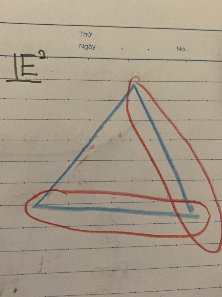
We can now transition into another key definition which will help us apply quasi-isometries to metric spaces more concretely. We will introduce geodesic spaces which will serve as tools, eventually bringing us to a very intriguing lemma. We first introduce the geodesic triangle, pictured below. This figure consists of 3 vertices connected by three geodesics, $\alpha, \beta,$ and $\gamma$ .

A geodesic triangle with sides $\alpha, \beta, \gamma$ and the respective neighborhoods.

Definition A geodesic triangle is $\delta$ -slim if $\alpha$ is contained in the $\delta$ -neighborhood of all sides.
Explicitly,
$ \alpha\subseteq N_{\delta}(\beta\cup \gamma)$

$\beta\subseteq N_{\delta}(\alpha\cup \gamma)$

$\gamma\subseteq N_{\delta}(\beta\cup \alpha)$
Furthermore, a geodesic metric space is $\delta$ -hyperbolic if all geodesic triangles are $\delta$ -slim.

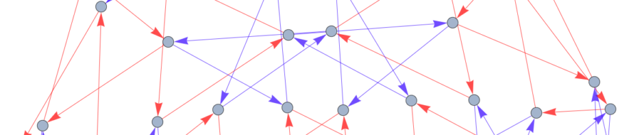
In order to understand this, what we really need are some pictures of groups. Below we draw a tree, $T$ , a structure which is classified as 0-hyperbolic. The $\delta=0$ means that the neighborhoods are perfect unions of each other, cyclically as described in the formula.

A tree with three neighborhoods of $\alpha, \beta, \gamma$ .

Similarly, we can draw the graph for $\mathbb{Z}_3*\mathbb{Z}_4$ , which is not a tree, and is anywhere from 1-hyperbolic to 4-hyperbolic, depending on the choice of $\delta$ -neighborhoods.

The $\mathbb{Z}_3*\mathbb{Z}_4$ with neighborhoods $\alpha, \beta, \gamma$ .

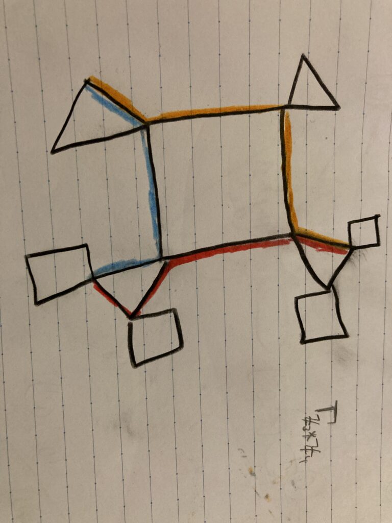
In terms of metric spaces, we say that if metric space $X$ has a bounded diameter then it must be $\delta$ -hyperbolic. This is fairly intuitive since we can will any bounded space with geodesic triangles and achieve our goal. However, the Euclidean space $\mathbb{E}^2$ is not $\delta$ -hyperbolic and thus neither is $\mathbb{Z}^2$ . We provide a figure of $\mathbb{E}^2$ to show that we cannot form a valid geodesic triangle in this space.

The non-example of $\mathbb{E}^2$ as a $\delta$ -hyperbolic space.

As promised, we can consider other geodesic shapes, other than triangles. For instance, we introduce the geodesic quadrilateral with sides $\alpha, \beta,\gamma,$ and $\omega$ . Similarly to the triangle, the quadrilateral is $2\delta$ -slim if $\alpha\subseteq N_{\delta}(\beta\cup \gamma\cup \omega)$ , and so on, in a cyclic fashion for all geodesics. We also note that there exist two points on opposite sides of the quadrilateral, such that $d(p_1,p_2)<2\delta$ , as shown below.

The geodesic quadrilateral with sides $\alpha, \beta, \gamma, \omega$ and proper $\delta$ length limits.

The geodesic quadrilateral with sides $\alpha, \beta, \gamma, \omega$ and proper $\delta$ length limits.

Notice that what we really are doing here is triagonalizing a quadrilateral. Thus in a similar fashion we can triagonalize any $n$ -gon with less than or equal to $n-2$ geodesic triangles.

We also introduce a puzzle to the reader: generalize the following neighborhood mapping on the quadrilateral to an $n$ -gon.

We now state this formally as a theorem.

Theorem If $X$ is $\delta$ -hyperbolic, then geodesic quadrilaterals are 2 $\delta$ -hyperbolic. Furthermore, on a geodesic quadrilateral there exist opposite edges such that $d(x,y)<2\delta$ .

We now transition slightly towards nearest point projections, which are a common topic in the geometry in the Euclidean space. However, this is not well defined in hyperbolic geometry. To aid this, we will introduce a lemma.

Lemma Let $\gamma$ be a geodesic in hyperbolic space and let $p\notin\gamma$ . If $q, q'$ are two points that realize the minimum distance from $p$ to $\gamma$ , then $d(q,q')\leq 4\delta$ .

We will prove this by contradiction, supposing that $d(q,q')> 4\delta$ and using the triangle inequality for metrics in order to show that this cannot be the case.

Proof Suppose $d(q,q')> 4\delta$ . Then since $q,q'$ do realize the minimum distance between some point $p\notin\gamma$ and $\gamma$ , there exist $q,q'\in \gamma$ such that $d(p,\gamma)=d(p,q)=d(p,q')$ . Now recall that $\gamma$ is a geodesic and thus there esists some $w\in\gamma$ such that $d(w,q), d(w,q')<2\delta$ . (See the picture below!) Since $\gamma$ is a hyperbolic space, we can reason that the triangle with vertices $pqq'$ is $\delta$ -hyperbolic and thus, without any loss of generality, there exist some $z$ on the line segment $qp$ such that $d(z,w)<\delta$ .

Combining the steps together and using the triangle inequality, we get a chain of inequalities
$d(q,z)>d(q,w)-d(w,z)>2\delta-\delta>\delta.$

Now, using the triangle inequality once more, we find
$d(p,w)<d(p,z)+d(z,w)<d(p,z)+\delta<d(p,z)+d(z,q)=d(p,q),$
which implies that $w$ is the closest point on $\gamma$ to $p$ which contradicts our original assumption. We thus conclude that $d(q,q')\leq 4\delta$ .

Figure to go with the proof of the lemma

This gives us a method of finding closest points to a space in hyperbolic-space. Metrics prove extremely useful for our purposes, and then lovely triangle inequality is key for our conclusions. Several corollaries follow, one of which I will state here for the purposes of motivation to future classes.
Corollary If $\gamma'$ is a geodesic segment which is ‘far away’ from another geodesic 4 $\gamma$ . Then the projection of $\gamma'$ onto $\gamma$ has diameter $\leq10\delta$ .

A similar approach to the closest point lemma is valuable for this theorem and a useful representation of the concept is shown below.

Two geodesic segments $\gamma, \gamma'$ projected onto eachother.

With this we conclude our blog post, with excitement of seeing what comes next in the world of the hyperbolic space and geodesics. It will be intriguing how hyperbolic groups fit in with all of these new theorems and techniques, leading us to satisfactory group representations in hyperbolic space. Other lemmas are soon approaching as well — such as the wonderful Morse lemma!

3 Responses to Wednesday Week 7: More hyperbolic spaces!

Horace Fusco says:

October 31, 2022 at 6:40 pm

Thank you for spelling out all the triangle inequalities so carefully. I feel like when you do this type of math there’s almost an extra little voice that’s got to be back there somewhere reminding you to use the triangle inequality–because it’s such a reasonable thing but it’s so easy to forget how powerful it can be. I think of it like the geometric pigeonhole principle.

Michaela Polley says:

November 8, 2022 at 7:59 pm

Nice post! In your proof of the lemma regarding two nearest point projections being at most 4 $\delta$ apart, I think you flipped the inequality sign for the distance between $w$ and $q$ and $w$ and $q'$ (your picture is correct!). Otherwise, looks really good! I appreciate all of the very carefully drawn diagrams and explanations.

Shuhang Xue says:

November 13, 2022 at 6:10 pm

Good post! I want to comment on another statement for the last corollary. Indeed, I would phrase it as if we have a geodesic rectangle, then one of the four edges has a distance of less than 10 $\delta$ . The reason behind this revision is that I do not need to define what it means to be “far-away” so that the statement is more useful.

We cannot be sure whether the $2\delta$ narrowing behavior happens along the projection or the two original geodesics. If it is the first situation, then the proof goes exactly as Osip mentioned. If it is the latter situation, then we may think about the two original geodesics as projections and apply the argument again.

3 Responses to Wednesday Week 7: More hyperbolic spaces!

Leave a Reply Cancel reply

Recent Posts

Recent Comments