Wednesday Week 7: More hyperbolic spaces!

Introduction

Last class, wonderfully recounted by Michaela, we learned about hyperbolic groups and defined the terms quasi-isometry and quasi-isometric. Importantly, we showed that there is a quasi-isometry between any group and its Cayley graph, and that two Cayley graphs of the same group are always quasi-isometric. In today’s class we continued with a similar subject matter, focusing in on quasi-isometries. We will first present the theorem that quasi-isometries are equivalence classes on metric spaces with the motivation that quasi-isometries are able to preserve the hyperbolic structure of a group. Subsequently, we will define and discuss what it means to be \delta-slim, showing several neat examples through figures.

We begin with a definition which was given last class and will prove essential in our discussion today.

Definition The mapping f:X\longrightarrow Y is (K,\epsilon)-quasi-isometric if
<em>\frac{1}{K}d_x(x,y)-\epsilon\leq d_y(f(x),f(y))\leq K d_x(x,y)+\epsilon.</em>
Furthermore, if f is a quasi-isometry, then f(X) is a net in Y.

The definition is key to our purposes since it constrains how the metrics of the two spaces X and Y can move around.

We can now go ahead and state the aforementioned theorem about quasi-isometries as equivalence classes.
Theorem The relation quasi-isometry on metric spaces is an equivalence relation.

The proof is simple for the most part, although some of it will be left for our upcoming homework.
We provide a brief sketch of the proof, covering the three attributes needed for an equivalence class. However, we will omit the computation for the symmetric case since it is not essential to our theme of the class.

Reflexivity, is fairly trivial since the identity is a quasi-isometry. Transitivity requires a brief calculation, which is left for our homework. Finally, the symmetric part is a bit more involved. We first define a quasi-isometry f:X\longrightarrow Y. For all y\in Y, there exists x_y\in Y such that d(f(x_y),y)< R, for some real number R.
From here we define g:Y\longrightarrow X where g(y)=x_y and the metric d(f(x_y),y)<R. The mapping g is the quasi-inverse and for f to be quasi-isometric we must have g be quasi-isometric. In search of a contradiction, we claim that g is not quasi-isometric and use the previous definition to constrain the metric, leading us to a contradiction.

Before we move on to \delta-slim content, it is essential to note what quasi-isometries are good for. As we may have noticed, they are very loose, which may give reason for worries. However, they are the perfect equivalence relations for some spaces, namely, in hyperbolic geometry. On the other hand, quasi-isometries are not so useful in Euclidean space.

We can now transition into another key definition which will help us apply quasi-isometries to metric spaces more concretely. We will introduce geodesic spaces which will serve as tools, eventually bringing us to a very intriguing lemma. We first introduce the geodesic triangle, pictured below. This figure consists of 3 vertices connected by three geodesics, \alpha, \beta, and \gamma.

A geodesic triangle with sides \alpha, \beta, \gamma and the respective neighborhoods.


Definition A geodesic triangle is \delta-slim if \alpha is contained in the \delta-neighborhood of all sides.
Explicitly,

<em> \alpha\subseteq N_{\delta}(\beta\cup \gamma)

<em>\beta\subseteq N_{\delta}(\alpha\cup \gamma)

<em>\gamma\subseteq N_{\delta}(\beta\cup \alpha)
Furthermore, a geodesic metric space is \delta-hyperbolic if all geodesic triangles are \delta-slim.

In order to understand this, what we really need are some pictures of groups. Below we draw a tree, T, a structure which is classified as 0-hyperbolic. The \delta=0 means that the neighborhoods are perfect unions of each other, cyclically as described in the formula.

A tree with three neighborhoods of \alpha, \beta, \gamma .

Similarly, we can draw the graph for \mathbb{Z}_3*\mathbb{Z}_4, which is not a tree, and is anywhere from 1-hyperbolic to 4-hyperbolic, depending on the choice of \delta-neighborhoods.

The \mathbb{Z}_3*\mathbb{Z}_4 with neighborhoods \alpha, \beta, \gamma.

In terms of metric spaces, we say that if metric space X has a bounded diameter then it must be \delta-hyperbolic. This is fairly intuitive since we can will any bounded space with geodesic triangles and achieve our goal. However, the Euclidean space \mathbb{E}^2 is not \delta-hyperbolic and thus neither is \mathbb{Z}^2. We provide a figure of \mathbb{E}^2 to show that we cannot form a valid geodesic triangle in this space.
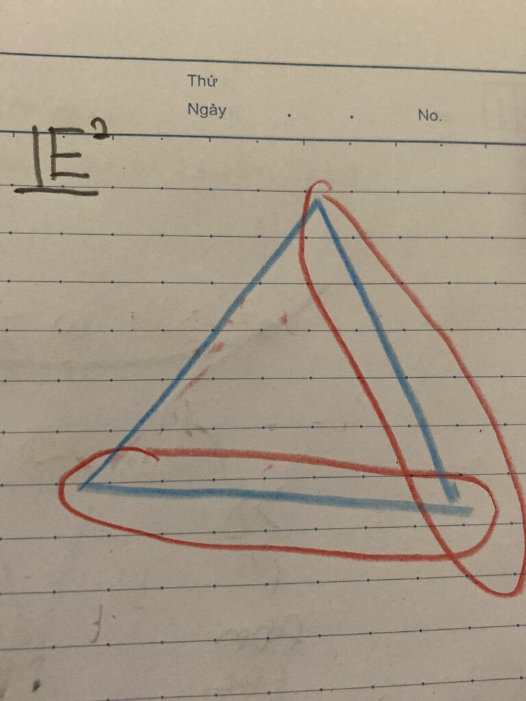
The non-example of \mathbb{E}^2 as a \delta-hyperbolic space.

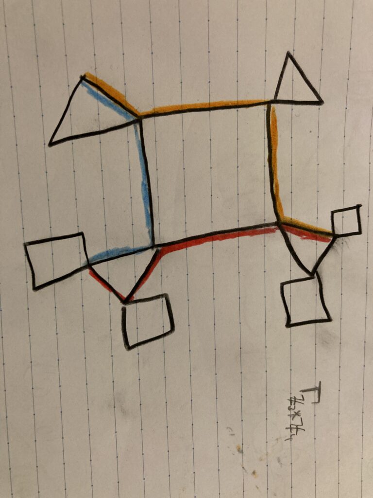
As promised, we can consider other geodesic shapes, other than triangles. For instance, we introduce the geodesic quadrilateral with sides \alpha, \beta,\gamma, and \omega. Similarly to the triangle, the quadrilateral is 2\delta-slim if \alpha\subseteq N_{\delta}(\beta\cup \gamma\cup \omega), and so on, in a cyclic fashion for all geodesics. We also note that there exist two points on opposite sides of the quadrilateral, such that d(p_1,p_2)<2\delta, as shown below.

The geodesic quadrilateral with sides \alpha, \beta, \gamma, \omega and proper \delta length limits.

Notice that what we really are doing here is triagonalizing a quadrilateral. Thus in a similar fashion we can triagonalize any n-gon with less than or equal to n-2 geodesic triangles.

We also introduce a puzzle to the reader: generalize the following neighborhood mapping on the quadrilateral to an n-gon.

The puzzle!

We now state this formally as a theorem.

Theorem If X is \delta-hyperbolic, then geodesic quadrilaterals are 2\delta-hyperbolic. Furthermore, on a geodesic quadrilateral there exist opposite edges such that d(x,y)<2\delta.

We now transition slightly towards nearest point projections, which are a common topic in the geometry in the Euclidean space. However, this is not well defined in hyperbolic geometry. To aid this, we will introduce a lemma.

Lemma Let \gamma be a geodesic in hyperbolic space and let p\notin\gamma. If q, q' are two points that realize the minimum distance from p to \gamma, then d(q,q')\leq 4\delta.

We will prove this by contradiction, supposing that d(q,q')> 4\delta and using the triangle inequality for metrics in order to show that this cannot be the case.

Proof Suppose d(q,q')> 4\delta. Then since q,q' do realize the minimum distance between some point p\notin\gamma and \gamma, there exist q,q'\in \gamma such that d(p,\gamma)=d(p,q)=d(p,q'). Now recall that \gamma is a geodesic and thus there esists some w\in\gamma such that d(w,q), d(w,q')<2\delta. (See the picture below!) Since \gamma is a hyperbolic space, we can reason that the triangle with vertices pqq' is \delta-hyperbolic and thus, without any loss of generality, there exist some z on the line segment qp such that d(z,w)<\delta.

Combining the steps together and using the triangle inequality, we get a chain of inequalities
d(q,z)>d(q,w)-d(w,z)>2\delta-\delta>\delta.

Now, using the triangle inequality once more, we find
d(p,w)<d(p,z)+d(z,w)<d(p,z)+\delta<d(p,z)+d(z,q)=d(p,q),
which implies that w is the closest point on \gamma to p which contradicts our original assumption. We thus conclude that d(q,q')\leq 4\delta.

Figure to go with the proof of the lemma

This gives us a method of finding closest points to a space in hyperbolic-space. Metrics prove extremely useful for our purposes, and then lovely triangle inequality is key for our conclusions. Several corollaries follow, one of which I will state here for the purposes of motivation to future classes.
Corollary If \gamma' is a geodesic segment which is ‘far away’ from another geodesic 4\gamma. Then the projection of \gamma' onto \gamma has diameter \leq10\delta.

A similar approach to the closest point lemma is valuable for this theorem and a useful representation of the concept is shown below.

Two geodesic segments \gamma, \gamma' projected onto eachother.

With this we conclude our blog post, with excitement of seeing what comes next in the world of the hyperbolic space and geodesics. It will be intriguing how hyperbolic groups fit in with all of these new theorems and techniques, leading us to satisfactory group representations in hyperbolic space. Other lemmas are soon approaching as well — such as the wonderful Morse lemma!

Posted in Uncategorized | 3 Comments

Week 7 Monday: Hyperbolic Groups and Quasi-Isometry

Hyperbolic Groups

The next thrust of the course is hyperbolic groups. We care about hyperbolic groups for four reasons:

  1. In many models of “random groups,” groups are hyperbolic with probability 1. For example, under the few-relators model of random groups, where we pick relators at random given a set of generators, as the allowed length of relators goes to \infty, the probability of the group generated being hyperbolic goes to 1.
  2. All free groups and finite groups are hyperbolic.
  3. All hyperbolic groups are automatic.
  4. Hyperbolic groups have an exceptionally nice solution to the word problem.

We will now give the definition of a hyperbolic group, acknowledging that there are two words that we have not previously defined.

Definition. A group G is hyperbolic if it acts geometrically on a \delta-hyperbolic space.

From the motivating facts above, one might think that it is very difficult to find groups that are not hyperbolic! This is in fact not the case. For exception, any group which contains \mathbb{Z}^2 (including \mathbb{Z}^2 itself) is not hyperbolic. Additionally, the Baumslag–Solitar groups are also not hyperbolic. We don’t have the tools yet to show that these are not hyperbolic, they just serve as examples to show that not every group we know about falls under this new categorization.

Next, we will discuss isometries and quasi-isometries, which we will need when thinking about \delta-hyperbolic spaces.

Isometries

We begin by reviewing the definition of a metric space.

Definition. A metric space is a set X along with a metric on X, d_x : X\times X \rightarrow \mathbb{R}_{\ge 0} such that the metric satisfies three conditions:

  1. d_x(x,y)=0 if and only if x=y,
  2. d_x(x,y)=d_x(y,x) , and
  3. d_x(x,y) + d_x(y,z) \ge d_x(x,z).

Then,

Definition. An isometry is a map from one metric space to another (or itself) that preserves distances. That is,

f: X \rightarrow Y such that d_x(x,y)=d_y(f(x),f(y)).

Additionally,

Definition. Two spaces, X and Y, are isometric if there exists a surjective isometry from X to Y.

Let us now consider a couple of examples. We know that mathbb{E}^2 (\mathbb{R} with the Euclidean metric) is a metric space. Isometries of \mathbb{E}^2 to itself include reflections, rotations, and translations. Non-Isometries of \mathbb{E}^2 to itself include projection onto a line, shearing, and scaling since none of these preserve distance between points. Consider as well the map from \mathbb{R} to \mathbb{E}^2 defined by x \rightarrow (x,0). While this map is an isometry, the two spaces are not isometric since the mapping is not surjective and no such surjective mapping exists. While it “feels” right that the real number line and the Euclidean plane are not isometric (they have different dimensions for starters), actually showing that they are not isometric is much more difficult and beyond the scope of this blog post.

Our overall goal is to define some sort of relationship so that a group G would be “equivalent” to its Cayley graph. How to go about doing this is not immediately obvious, since G is a group that does not depend on the choice of generating set and the Cayley graph is a graph that does depend on the choice of generating set. In order to do this we will massage the definition of an isometry and define a quasi-isometry and what it means for two spaces to be quasi-isometric. This is a common practice in math: if a definition isn’t working the way you want it to, loosen the definition slightly and hope that you aren’t loosening it so much that it is no longer useful.

Quasi-Isometries

Many of the spaces we will be interested in studying will be graphs, thus it will be helpful to define a metric for graphs before diving into the heart of quasi-isometries.

Let \Gamma be a graph and let us induce a metric on \Gamma by path length. We can think of each edge as an isomorphic copy of the interval [0,1]. We want to think of the edges like this so that we can define any point between two vertices. For any given path between two vertices, we will set the starting vertex as zero and then build the path up, with each vertex we pass adding a total of one to the path and following edges only partially resulting in adding the corresponding fraction of one to the path. We then define the metric d_\Gamma(x,y) to be the infimum of the set of path lengths of all possible paths between x and y. Checking that d_\Gamma(x,y) is in fact a metric is straightforward and left as an exercise to the reader. Let us now formally define path.

Definition. A path of length L is an isometric embedding of [0,L] on X.

The paths we will care most about are those of minimum length:

Definition. A geodesic is a path of minimum length. Additionally, a metric space is called geodesic if all pairs of points can be connected with a geodesic.

For example, \mathbb{E}^2 and \Gamma with the path metric are both geodesic. However, if we remove the origin from \mathbb{E} we no longer have a geodesic. Consider a point on the negative x-axis and a point on the positive x-axis. In order to connect them with a path of minimum length we would need to go through the origin. Given any path that went around the origin, we would always be able to find a shorter path that got closer to the origin and would thus be shorter. Hence, the space is not geodesic.

We have now formally established graphs as metric spaces and can consider their isometries. Recall that our goal was to find some sort of equivalence between a group and its Cayley graph (with respect to some generating set). We know that this relationship cannot simply be being isometric, since G is always countable and \Gamma_{G,S} is always uncountable (every edge is isometric to [0,1] which is itself uncountable). Thus, there will be no surjective mapping from G to \Gamma_{G,S}. We will fix this problem by loosening our definition of isometry, beginning with the subjectivity requirement.

Definition. A net in a metric space X is a subset P \subseteq X such that N_R(P)=X for some R\ge 0 and R being finite.

Essentially, a net is a subset of points in the metric space which are spread out enough around the space, so that if we blur the edges of the net (take some finite neighborhood around each point in P), we get the whole set X. Hence, it doesn’t make sense to talk about the net of a finite set, since we can simply pick any point x\in X that pleases us and then set R to be large enough to cover the whole set X.

The idea of a net allows us to define a mapping f from G to \Gamma_{G,S} where f(G) is the set of vertices of the Cayley graph and thus f(G) is a net is \Gamma_{G,S}. However, now we don’t have inverses. We fix this by loosening our definition in a slightly different way:

d_x(x,y)-\epsilon \le d_y(f(x),f(y)) \le d_x(x,y) + \epsilon.

This statement says that the distance under the mapping is “close enough” to the distance in the original metric space where there is some sort of fudge factor which works for all pairs of points x,y.

Finally, using this additive fudge factor and adding in a multiplicative fudge factor to account for variations between generating sets of groups, we get our definition of quasi-isometric and quasi-isometry.

Definition. If X,Y are metric spaces, f: X\rightarrow Y is (K,\epsilon)-quasi-isometric if

\frac{1}{K} d_x(x,y) - \epsilon \le d_y(f(x),f(y)) \le Kd_x(x,y)+\epsilon.

Furthermore, if f(X) is a net in Y, then f is a quasi-isometry.

Notice that this definition doesn’t quite mirror the definition of isometry/isometric. In fact, the distance-preserving relationship falls under quasi-isometric and isometry and the additional requirement of being surjective-(ish) falls under being isometric and being a quasi-isometry.

This achieves our goal! There is a quasi-isometry between a group and its Cayley graph, and two Cayley graphs of the same group are quasi-isometric. Next time we will show that being quasi-isometric is an equivalence relation on metric spaces.

Sources:

https://en.wikipedia.org/wiki/Random_group

https://en.wikipedia.org/wiki/Hyperbolic_group

Posted in Uncategorized | 2 Comments

Week 6 Friday: The Grigorchuk Group and its Friends

Introduction

This Friday we went international with a captivating lecture on the Grigorchuk Group and its good buddies given by guest lecturer Professor Rachel Skipper all the way from École Normale Supérieure in Paris!

The Automorphisms of the Infinite Binary Rooted Tree

We’ll get to the Grigorchuk group in a bit, but let’s first start off with a group somewhat adjacent to it in its construction and motivation. We’d like to characterize some of the automorphisms of an infinite binary rooted tree (shown below).

a rooted binary tree

I’ve labelled the vertices to help us when we consider automorphisms of this tree (symmetries that preserve gluing). With some experimentation, we can see that one valid symmetry could be swapping two branches that share a node above it. However, since this symmetry has to preserve gluing, every part below must also get swapped. It’s like a domino effect! I think this hints at the recursive nature of elements in this group. Let’s characterize these more rigorously now.

We have the group G = \langle a, b, c \rangle generated by three elements:

a = (c,b) \sigma
b = (b,c) \sigma
c = (a,a)

Where \sigma = (01) is a transposition, note that is it 2-torsion! This notation is a little bit confusing at first, but I hope to make it clear through a diagram. If we apply a to our tree, we change the labels as follows. The smaller arrows represent the swapping at that level.

our tree with a applied to it. as we can see, there’s a cascade!

When we multiply these generators, we are able to move the permutations across the ordered pairs ‘at the cost’ of applying the permutation to the ordered pair. For instance, we have

a \cdot b = (c,b) \sigma (b,c) \sigma
a \cdot b = (c,b)(c,b) \sigma \sigma
a \cdot b = (c^2,b^2)

So the multiplication in the ordered pairs is carried out component wise and we multiply the permutations as usual.

Mealy Automata

As it turns out, a finite state automaton is able to capture this information in a really nice way for us. We define a Mealy automaton as a 4-tuple. Its four components are

  • Q, a finite set of states
  • X, a finite alphabet
  • \lambda, a function Q \times X \rightarrow X called the output function
  • \tau, a function Q \times X \rightarrow Q called the transition function

This is a little different from the automata we’ve seen before, as our vertices hold more meaning and our edges are labelled a little differently. Again, we make this clear with an example.

the Alëshin automaton

Let’s write out the components of this Mealy Automaton:

  • Q = {a,b,c}
  • X = {0,1}
  • \lambda, a function Q \times X \rightarrow X is defined by following the arrow and seeing what element of X corresponds to it on the edge. For example, \lambda (a,0) = 1
  • \tau, a function Q \times X \rightarrow Q is defined similarly as above, except instead of the edge label, our value is the state the arrow leads to. For example, \tau(a,0) = c

This automaton is called the Alëshin automaton, and describes the generators above! Here’s how: recall we have a = (c,b) \sigma. When we look at our machine, we see two arrows out of a. The edge labels indicate the permutation and the destinations indicate what goes in the ordered pair. One arrow to c has the label 0|1. The 0 indicates that c is in the first entry of the ordered pair, and the 0|1 indicates that 0 goes to 1.

So, these machine gives us an exact way of transforming strings of 0s and 1s with our states. This is powerful! Remember these strings correspond to vertices in our tree, so this allows us to see exactly where a vertex goes under some symmetry. We just have to follow each step, with our output and transition functions! Let’s try it with 0110 under a.

a0110
(a0)110
(1c)110
1(c1)10
1(1a)10
11(a1)0
11(0b)0
110(b0) – we reach the end of our string so no more state in our output
1101 \leftarrow this is where 0110 ends up under the transformation a

Note the multiplication and the ‘cost of moving an ordered pair across’ shows up here too! Fun fact: the group generated by a,b,c is actually free! This was proven once by Aleshin, but that proof was lacking. As noted by Professor Skipper, it was proven properly by Vorobets and Vorobets in 2007. This paper is pretty readable!

The Grigorchuk Group

We’ve now developed enough machinery to talk about the Grigorchuk group! Like the group above, it is most nicely described a Mealy automaton (shown below).

the Mealy automaton representing the Grigorchuk group

Like the group above, it can also be visualized as acting on a rooted binary tree. See below!

the generators acting on the tree courtesy of Wikipedia

It is generated by the four elements (depicted above and written out below). Here, e represents the group identity

a = (e,e) \sigma
b = (a,c)
c = (a,d)
d = (e,b)

The Grigorchuk group has some interesting properties! One being that is it a finitely generated, infinite torsion group. What’s more is that every element has order of a power of 2! Pretty crazy stuff. I’m not going to include a full proof here, but instead walk through an part of an example to maybe convince you of that last fact.

We can do computations to obtain

a^2=b^2=c^2=e
bc = cb = d
cd = dc = b
bd = db = c

This means that we are able to write every element as an alternating product of as and other generators. More computation gives us

aba = (c,a)
aca = (d,a)
ada = (b,c)

Can you see where this is going? Let’s do an explicit example.

We’d like to verify that (ab)^{16}=1

abababababababababababababababab
(aba)a(aba)a(aba)a(aba)a(aba)a(aba)a(aba)a(aba)a
(c,a)(a,c)(c,a)(a,c)(c,a)(a,c)(c,a)(a,c)(c,a)(a,c)(c,a)(a,c)(c,a)(a,c)(c,a)(a,c)
(caca...,acac...)

This is getting a little tiring to write, but at the end we are able to get down to a bunch of b^2 elements which are just the identity. I’m cutting this part just a little short because I’m really excited about the next section, but if you’re interested you should check out Chapter 6 in our book. The group there is the Gupta-Sidki group, which is similar (it looks at symmetries of an infinite rooted ternary tree). Professor Skipper noted that most of our present day finitely generated infinite torsion groups (more accessible ones anyways) come from groups adjacent to the Grigorchuk group!

The Hanoi Towers Group

Speaking of infinite rooted ternary trees, we can use them to play (and beat) Hanoi! Ternary makes sense in the case of three pegs, as we can make at most 3 swaps at any moment. Let’s construct our automaton to help us.

  • three pegs, labelled 1,2, and 3
  • three nontrivial states representing possible moves between the pegs
  • a string representing the current location of the discs
here’s an example of the string and how it changes. this example uses 0,1,2 labels instead of 1,2,3

Note that this automaton codes in valid moves! I think that’s super cool! This automaton can actually tell us a lot more than just then 3 disc case, but let’s just consider the 3 disc case for now.

A graphical method of presenting this case is a Schreier graph. Informally, it is a way of capturing information about a self-similar group at a certain level. To give an example, look at this automaton called the Adding Machine.

The Adding Maching automaton

We can see it acting on an infinite binary rooted tree below. The * represents a swap, and the plain vertex indicates nothing (the identity).

the Adding Machine on a tree

As we can see on the tree, there are distinct ‘levels’! To construct a level n-Schreier graph, we take the vertices of that level to be the states, and all the nontrivial states to be our directed edges.

Level 2 Scheirer graph for the Adding Machine
Level 3 Scheirer graph for the Adding Machine

As you might guess (and hinted at from the name) the group associated with the adding machine is actually \mathbb{Z}, the infinite cyclic group.

Now back to our Tower of Hanoi! Let’s look at our Level 3 Schreier graph.

The graph clearly shows the quickest way to win (just 7 moves) is from the state 111 to 333! One thing that really stands out to me is that this graph will show you how to get to any state. Another thing MurphyKate mentioned was that as we keep increasing the level, our Schreier graph will resemble the Sierpinski triangle!

Thank you for reading! A lot of the last section was from the book A Sampling of Remarkable Groups written by Bonanome, Dean and Dean.

Posted in Uncategorized | 4 Comments

Solving the Word Problem

We left off our discussion of regular languages with dashed hopes when we learned that \textrm{Null} (G) is a regular language if and only if G is finite. This means that dealing with \textrm{Null} (G), the set of words on the generators of G which are trivial in G, will never help us resolve the word problem because if G is finite, we already know we can solve the word problem with the Cayley graph!

Fortunately all is not lost. The new plan of attack is to identify the situations in which a normal form for some group G is also a regular language. In these cases we may be able to use some set of FSA’s to relate a word on the set of group generators to the normal form for the group element that the word reduces to (although ultimately, as we will see, we won’t even need an FSA that accepts a normal form for G).

First we should see an example of a group with a normal form which is also a regular language.

Definition: A regular normal form of a group G is a normal form which is also a regular language.

Example:

Let G = \mathbb{Z} \times \mathbb{Z} = \langle a, b | ab = ba \rangle. We can set a normal form for this group, namely

NF = \{ a^n b^m | n , m \in \mathbb{Z} \}.

It is possible to build an FSA that accepts exactly this set as its language, illustrated below.

With this concept in hand, we can formulate a few interesting results.

Theorem: If G and H both have a regular normal form then so do G \times H and G * H.

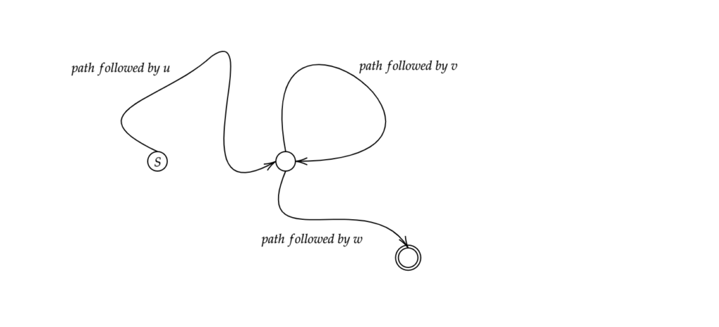
The proof will be assigned, so suffice it to say that it involves some ideas about combining regular languages that we’ve seen before. Before moving on to the word problem, we can squeeze a little more juice out of the concept of a regular normal form. A regular language is, for lack of a more appropriate phrase, a set of words which has a high degree of structural regularity. For this reason we suspect that a group which permits a normal form with this structure is “nice” in some basic way. For one thing, the set of nodes and edges in an FSA is finite, so every regular language will be finite or will have to somehow make use of cycles in the graph of its FSA. To put this into rigorous terms, we recall the pumping lemma.

Theorem (The Pumping Lemma): Let \mathcal{L } be regular, then there exists n \geq 1 such that for all words x \in \mathcal{L} with |x| > n, we can find u, v, w with |u|, |w| < n such that x = uvw and u v^i w \in \mathcal{L} for all i \in \mathbb{N}.

The proof worked via pigeonhole by setting n = \left| v( \mathcal{M} ) \right|, where \mathcal{M} is the FSA that accepts \mathcal{L}.

With this in mind we note that if G is in infinite group with a regular normal form, then we can use the cycles in the corresponding FSA to generate an element of G with infinite order.

Theorem: If G has a regular normal form and G is infinite, then G contains an element of infinite order.

Let \mathcal{M} be the FSA representing G. Let g \in G satisfy | g | > | v ( \mathcal{M} ) |. Here the absolute value sign denotes the word length of the representative of g in the regular normal form. We may take a word whose word length is greater than any integer, specifically | v ( \mathcal{M} ) |, because G is infinite and therefore its normal form is infinite. Let \pi: S^* \to G be the natural transformation that sends words to group elements. By an argument much like the proof of the pumping lemma, we note that the path which yields the word for g must contain a loop, therefore we have

    \[ g = \pi(uvw) .\]

Where u is given by a path from the start state to some vertex, \alpha, v is a loop that starts and ends at \alpha, and w is a path that begins at \alpha and ends at some accept state. We can see that u v^i w must also be accepted for all i \in \mathbb{N}, so because this language is a normal form, we have that for i > 1,

    \[ \pi(uvw) \neq \pi(u v^i w). \]

Since \pi is a homomorphism, we then have

    \[ \pi(v) \neq \pi(v^i) = \pi(v)^i .\]

This means that the element \pi(v) must have infinite order, which is all to say that if G has a regular normal form, then G is not infinite torsion.

Permitting a regular normal form is a great property for a group to have, but we already get the feeling that it is quite specific, and it is possibly difficult to prove whether a group even has it. We will not use these normal forms explicitly in our solution of the word problem, but we will retain the general idea of making an FSA work for us to produce words with useful properties. This is part of what motivates the following definition.

Definition: Let G = \langle S | R \rangle be a group. We say G has an automatic structure if there exists the following set of FSAs

  • \mathcal{M}_G where the language \mathcal{L}_G surjects onto G under \pi, namely ever element of G is represented by some word. This is FSA is called the word acceptor.
  • \mathcal{M}_{=} where \mathcal{L}_{= } = \{ (u,v) | u,v \in \mathcal{L}_G, \pi(u) = \pi(v) \}. This FSA is called the equality checker.
  • \mathcal{M}_s where \mathcal{L}_s = \{ (u,v) | u,v \in \mathcal{L}_G, \pi(v) = \pi(us) \}. This is the word comparator.

A few examples are in order to unpack this definition. First we draw out all the FSA’s for the example G = \mathbb{Z}.

We have only drawn \mathcal{M}_a since \mathcal{M}_{a^{-1}} would look very similar. In general we do not necessarily have that the language given by \mathcal{M}_G is necessarily a normal form for G, but in this case we do, which means that drawing \mathcal{M}_{=} is easy as we can replace every edge a with the edge (a,a) and so on, since every word uniquely represents a group element, so \pi(u) = \pi(w) implies that u and w are the same word. We will see this at play in the next example, where G = F_2. Here we will omit \mathcal{M}_{=} since we understand it’s structure, and again only draw \mathcal{M}_{a} for reasons of symmetry.

Drawing \mathcal{M}_{a} once we have \mathcal{M}_{=} is not too large a task. In the above example, the orange part of the graph is exactly what \mathcal{M}_{=} would be, where the purple arrows turn this graph into the graph of \mathcal{M}_{a}. Further examples of groups with automatic structure include all free groups and all free abelian groups, all finite groups, many coxeter groups, all braid groups, hyperbolic groups, and the special linear group over \mathbb{Z} for n = 2. A few groups which do not have automatic structure are infinite torsion groups, special linear groups over \mathbb{Z} with n \geq 3, and most Baumslag-Solitar groups.

We are now in a position to exhibit the crown jewel of our discussion.

Theorem: If G is automatic then G has solvable word problem.

Let G = \langle S | R \rangle. Pick some accepted word u. For each letter x \in S, we will use the automata that make G automatic to find an accepted word for \pi(ux).

We take the word comparator automaton \mathcal{M}_x and observe that we can take it to have no two edges leaving the same vertex with the same label by arguments we’ve made before. By definition \mathcal{M}_x accepts pairs (v, u) such that \pi(u) = \pi(vx). Sweeping a few things under the rug, we argue that we can follow the path that gives (v, u) in \mathcal{M}_x and read off the word word v, where we are guaranteed \pi(v) = \pi(ux). This is an algorithm which gives us an accepted word for \pi(ux ).

The key idea is that we can use this algorithm generate an accepted word for every element of G. There is some word in the language \mathcal{L}_G which is the identity in G, so just take u to be this word. Now we can express every element of G as u x_1 \cdots x_n where x_i \in S are letters in our generating set. Note that \pi(u x_1 \cdots x_n ) = \pi(u) \pi( x_1 \cdots x_n ) = \pi(x_1 \cdots x_n ). We can apply the above algorithm iteratively, first to get an accepted word for the element \pi(u x_1 ), and after n repetitions to get the element \pi( u x_1 \cdots x_n ) = \pi(x_1 \cdots x_n ). Call this accepted word \omega. Since we know \pi(u) = e \in G, to solve the word problem we need to know if \pi(u) = \pi( \omega ). Fortunately we have a finite state automaton that tells us exactly this! We simply follow the path for (u , \omega ) and see if the pair is accepted.

Posted in Uncategorized | 3 Comments

Fifth Friday: Finding Further Fantastic Fun from Fabulous FSAs

On Wednesday, we learned about finite state automata (FSAs). An FSA is a finite, labeled, directed graph, whose vertices are called states, and whose edges are labeled with elements of a finite set called an alphabet. At least one vertex is designated a start state, and a subset of the vertices are designated accept states. An FSA accepts a string x if there exists a path labeled with the letters of x that connects the start state to an accept state. An FSA M accepts a language L if M accepts a string x if and only if x \in L.

A deterministic finite automaton (DFA) is an FSA with a unique start state, no two edges with the same label leaving the same vertex, and a label on every edge. A DFA is complete if, for every s \in S, every vertex has an edge leaving it labeled with s. A language is regular if there exists an FSA that accepts it. For any regular language L, there exists a complete DFA that accepts L.

We left off last class with some exercises regarding the closure properties of regular languages – if L and K are regular languages over the alphabet S, show the following are also regular:

  1. S^* - L (here, ^* is the Kleene star, meaning S^* is the set of strings consisting of letters from S). We denote this language L^{c} or L^{opp}.
  2. L \cup K
  3. L \cap K
  4. LK (the concatenation of L and K, or the set of strings xy where x \in L and y \in K)
  5. L \cup LL \cup LLL \cup...

Proof.

(1) If L is regular, there exists a complete DFA M_L that recognizes L. We construct a new complete DFA M' that is identical to M_L, but where any accept state in M_L is a non-accept state in M', and any non-accept state in M_L is an accept state in M'. Because M_L is complete, any string s \in S^* has a unique corresponding path from the start state to a state in M_L. That path ends at an accept state in M_L if and only if it does not end in an accept state in M'. Therefore, M' accepts the set of strings over S^* that are not accepted by M_L, which corresponds exactly to S^* - L.

(2) If L is regular and K is regular, there exist corresponding FSAs M_L and M_K that recognize L and K. We construct a new FSA M' that consists of M_L, M_K, and a new start state v that has a $-labeled edge to each of the vertices that was a start state in M_L or M_K. Then, M' consists of all strings recognized by M_L or by M_K, so it recognizes L \cup K, meaning L \cup K is regular.

(3) Closure under intersection follows from parts (1) and (2). Observe that:
L \cap K = L \cup K - [(L \cup K) - L] \cup [(L \cup K) - K]. Because regularity is preserved under taking complements and unions, it is also preserved under taking intersections.

(4) Because L and K are regular, there exist FSAs M_L and M_K that accept L and K. Construct a new FSA M' by drawing a $-labeled edge from each accept state of M_L to the start state of M_K, and making them non-accept states. The resulting language will accept any string x = \ell k where \ell \in L and k \in K.

(5) Because L is regular, there exists an FSA M that recognizes L. Draw $-labeled edges from each accept state of M to its start state to get a new machine M'. M' then accepts any string x^n for n \in \mathbb{N} where x \in L. These strings constitute the language L \cup LL \cup LLL \cup..., and M' recognizes it.

The above results give us lots of ways to show that a given language is regular, but how could we show that a language is not regular? For this, we’ll use an argument called the pumping lemma:

Theorem (pumping lemma for regular languages): Let L be a regular language. Then there exists an integer p \geq 1 such that, for every string x where |x| > p, there exist strings u, v, w such that:
1) x = uvw
2) uv^i w \in L for all i \in \mathbb{Z}_{\geq 0}
3) |u|,|w| < p

Proof. The proof is an application of the pigeonhole principle. Suppose a language L over S^* is regular. Then there exists an FSA M that accepts L. Consider a string x \in L such that |x| \geq |V(M)|. Consider the path \gamma_x in M whose edges trace out the letters in x. Because |x| \geq |V(M)|, there are at least |V(M)| edges in \gamma_x, so there must be at least |V(M)|+1 vertices. By the pigeonhole principle, at least one vertex is visited more than once. Therefore, there is a cycle along \gamma_x. Let v denote the word formed by the edges in this cycle, so v is a substring of x. Let u denote the prefix of x preceding v, and let w denote the suffix of x following v. Thus, x = uvw. It follows that any word uv^i w for i \in \mathbb{Z}_{\geq 0} is also accepted by M, as the paths traced out by u and w remain the same. Moreover, u and w must both be shorter than |V(M)|, which we choose to denote as p. This proves the lemma.

Illustration of the FSA M. When we “pump” v, we always get another word in L.

How can we use the pumping lemma in practice? We’ll use it to show that the language L = \{ a^n b^n | n \in \mathbb{N} \} is not regular.

Proof. We’ll use proof by contradiction. Suppose L is regular, so the pumping lemma holds for some sufficiently large integer p. Consider the string x = a^n b^n \in L for n \geq p. The pumping lemma tells us there exist strings u, v, and w such that x = uvw where |u|,|w| < p. Because |u|,|w| < p, u consists solely of a‘s, and v consists solely of b‘s. Moreover, v = a^\ell b^m for \ell, m>0. We contradict condition 2 of the pumping lemma, as for any i \geq 2, u v^i w \notin L.

Because I couldn’t help myself, I’ve outlined another way we can show \{ a^n b^n | n \in \mathbb{N} \} is not regular using the Myhill-Nerode theorem.

Theorem (Myhill-Nerode): Given a language L over the alphabet A, let _L \sim be an equivalence relation on A^* where x _L\sim y if there does not exist z \in A^* such that xz \in L and yz \notin L (or vice-versa). (This relation is sometimes called Nerode congruence). L is regular if and only if _L \sim has a finite number of equivalence classes.

I’ll forego a formal proof of the theorem here, but to get an intuition for why its true, note that (if L is regular) each equivalence class corresponds to a state in a minimum-size complete DFA recognizing L.

We can use the Myhill-Nerode theorem to show that L = \{ a^n b^n | n \in \mathbb{N} \} is not regular.

Proof. Consider the set of strings \{ a^n | n \in \mathbb{N} \}. Each strings a^k has a unique string b^k that can be appended to it to get a string in L. Therefore, each string in \{ a^n | n \in \mathbb{N} \} belongs to a unique equivalence class, so the Nerode congruence for L has an infinite number of equivalence classes. Thus, L is not regular.

At the end of Wednesday’s class, we discussed whether English is a regular language. While at the time I believed the answer was likely yes, I’ve since been convinced otherwise by some super interesting lecture notes from a course at UMass called Mathematical Linguistics, which itself borrowed the argument from the book Mathematical Methods in Linguistics, by Partee, ter Muelen, and Wall (page 480 in the pdf).

Here’s the essence of the argument: earlier, we showed that \{a^n b^n | n \in \mathbb{N} \} is not regular. A nearly identical proof can be used to show that \{a^n b^{n-1} c | n \in \mathbb{N} \} is also not regular. If we replace the letters a, b, and c with strings, the language remains non-regular. In particular, we’ll replace a with a noun (“the dog ”), b with a transitive verb (“chased ”), and c with a non-transitive verb (“got away”). Thus, we’re concerned with the language L = \{(“the dog ”)^n(“chased ”)^{n-1}(“got away”) | n \in \mathbb{N}\}.

I argue that this is a set of grammatically correct strings in the English language. If n=1, then the corresponding string is “the dog got away”, which is a valid English statement. If n=2, then the string is “the dog the dog chased got away” – in other words, the dog (who was being chased by another dog) got away. If n = 3, then we have the string “the dog the dog the dog chased chased got away. This means that the dog (chased by another dog, who was chased by a third dog) got away. If you believe this sort of nesting can go arbitrarily deep, then it follows that L is a subset of all English strings.

Here’s the trick: I will argue that the language K =  \{(“the dog ”)^i(“chased ”)^j(“got away”) | i,j \in \mathbb{N} \} is a regular language, recognized by the following FSA:
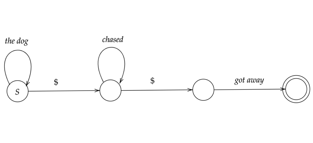
Let ENG denote the set of grammatically correct English strings. Suppose ENG is regular. Because ENG and K are both regular, it follows that ENG \cap K is regular. Observe that a statement of the form (“the dog ”)^i(“chased ”)^j“got away” only makes grammatical sense if j = i-1. Therefore, L = ENG \cap K. However, we know L is not regular! Thus, English is not a regular language.

Okay, I’ve gotten a bit carried away with formal language theory. Let’s get back to algebra.

Recall the word problem: given a presentation for a group G = \langle S | R \rangle and word w \in S^*, is it true that w =_G e? We say G has a solvable word problem if there exists an algorithm that correctly answers yes or no for any input w. Can we use FSAs to help us solve word problems for certain groups?

Here are a couple ideas:
1) We design an FSA that recognizes a language that consists of words in some normal form for a group. This could help us to solve the word problem for that group.
2) We define a language Null = \{ w \in S^* | \pi(w) = e \}. If Null is regular, then we can solve the word problem by plugging any word into our FSA for Null.

The first idea is one that we will explore (albeit with some modifications) next week when we talk about automatic groups. What about the second idea?

Unfortunately, it won’t do much for us. This is due to the following theorem.

Theorem: Null(G) is regular if and only if G is finite.

This means our idea can’t really help us, as we already know that any finite group has solvable word problem.

Proof (of Theorem). We will show implication in both directions.

( \impliedby ) Let G be finite. Then let the Cayley graph \Gamma_{G,S} be an FSA. Make v_e be the start state and the only accept state.

( \implies ) Assume Null(G) is regular. Let M be an FSA accepting Null(G).

We may assume that, for every vertex v \in V(M), there is a path from v to an accept state in M. To see why, note that if there is no such path, v is a “dead state,” so we may remove v (along with the subgraph that is reachable from v) to get an FSA that recognizes the same language as M.

Claim: |G| \leq |V(M)|.

Let w, w' be words in S^* such that the paths representing w and w' end at the same vertex v \in V(M). As mentioned above, we can assume that there is a path from v to an accept state. Let u be the string traced out by this path. Therefore, we have that:

\pi(wu) = \pi(w'u) = e
\pi(w)\pi(u) = \pi(w')\pi(u) = e
\pi(w) = \pi(w')

Therefore, if any two words trace out paths that end at the same state, they represent the same element of G. This implies the above claim, which implies G is finite, as any FSA has a finite vertex set. This concludes the proof.

In case it’s not clear already, I think that regular languages are really cool. They show up in lots of unexpected places (in formal linguistics, they form the base of the Chomsky hierarchy; in computer science, they encode decision problems that can be solved using finite amounts of memory). I’m super excited to see what role they play in geometric group theory.

Posted in Uncategorized | Tagged | 6 Comments

Wednesday Week 5: Automata

Introduction

Last class we discussed normal forms, which was wonderfully recapped in this Wednesday’s blog post by Akash. Today we will pretend that we are computer scientists and focus on languages and automata. Although it may seem a bit random at first glance, the motivations we have tie back into group theory and give us many useful new tools.

Motivations and Definitions

Several key terms in relation to today’s topic were introduced las class such as the alphabet : which is a set of words acted on by a monoid. A monoid is a group without any inverses.
We will focus on free monoid which implies that the elements within the monoid follow the structure of a free group. We can go further and motivate the need for languages.

Consider the monoid S and let S^* be the free monoid on S which contains all of the words coming from S.

Definition 1 A language on S is a subset \mathcal{L} of S^*.

From here we can go on to introduce today’s key topic: automata.

Definition 2
An automata on S is a directed graph with decorations.
1. Some vertices are labelled with a start state property.
2. Some vertices are labelled with a accept state property.
3.Some edges are labelled by elements of S.
4. Some vertices and edges are not labelled at all.

One may ask, well… how do we label these vertices? It’s easy! We must simply draw an S on each start vertex, a circle on each accept vertex, the element name on each labelled edge, and nothing at all in the case of the vertex or edge being unlabeled. We can also relate automata to languages since a possible way to create a language is to use an automaton. We can create a language from an automaton by observing all paths from a start state to an accept state, and reading off the edge labels.

Below is a simple example from class of an automata on S={a,b,c}. Notice, here the start state is also an accept state, which is fine since nowhere did we define them to be mutually exclusive.
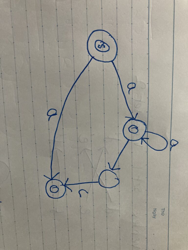
An Finite State Automaton

As we can see this looks pretty much like a directed graph with a few extra quirks… which we will get to in a second. We first connect it to languages. Given an automata \mathcal{M} there exists a language \mathcal{L}(\mathcal{M}) which is a graph of all paths from the start state to an accept state. For instance, in the example above we can find a finite set of elements which describe all possible paths from the start state to accept states of the automata. In the example above the language can be written as the set \mathcal{L}={1,a,a^n, a^nbc}, where n\in\mathbb{Z}^+ and is due to the loop edge connected to the top accept vertex. One of the most important things to notice from this example is the finiteness of \mathcal{L}. This will not always happen, but when it does it will be of utmost use to us. In fact, if \mathcal{M} is finite then we call it a finite state automata (FSA). The rest of our study for the course will be focused on finite state automata.

Before we go on further into more connected definitions, we pose a challenge question for the motivated reader.
Puzzle: Find an FSA, \mathcal{M}, such that \mathcal{L}(\mathcal{M})={ba^{3n}b^{-1}|n\in\mathbb{Z}} on the alphabet S={a,a^{-1}, b, b^{-1}}. How many can you find? Are there infinitely many possible options for alphabet to produce this automaton? How does this relate to Cayley graphs of some groups which we have seen in weeks prior?

We now move on to yet another addition to our vocabulary (no pun intended…).

Definition 3: An FSA is called deterministic if there exists a unique start state and no two edges leaving a vertex share the same label. Moreover, every edge must have a label in the DFA. A deterministic FSA is called DFA, for short.

We call a DFA complete if for every vertex in the automaton and each letter in the alphabet there are edges labelled by all letters leaving the vertex.

Claim: If \mathcal{M} is a DFA, then there exists \mathcal{M}' which is a completed DFA such that \mathcal{L}(\mathcal{M})=\mathcal{L}(\mathcal{M}'). We will not prove this for time’s sake but this could also be an additional puzzle that you can examine when your next class gets boring.

We have now covered the two main definitions of this blog post’s content. We now may ask the natural question … so what? We have FSAs and DFAs and we know how they are connected to monoids and alphabets and thus letters and words which we used prior. And yes, there seems to be a vague familiarity of the structure of automata and Cayley graphs of groups, however, we want a connection between all of it! Unfortunately we may not get to all of that today, yet, we will take the first step in connecting DFAs and FSAs more robustly in order to determine what languages can actually be generated or accepted by these new machines. The motivation is, roughly, the same as it has been for the entirety of the class. How can we reproduce something as a finite set of vertices and connecting edges where the path is structured by the specific decorations which we have described. Will the additional structure of automata help our quest of understanding infinite groups?

The key theorem, tied to this, that we will prove is as follows.

Theorem 1: The set of languages accepted by FSA are equal to the set of languages accepted by a complete DFA.

Wow! That’s really cool. I see this as a very useful path since an FSA seems like a very simple thing to construct, in general; and if we could then show that this same language can be accepted by a complete DFA, which has a more similar structure to some of the complicated groups we have seen, that would be really useful.

To motivate further we provide an example of a complete FSA on S={a,b,c} from which we will begin the proof. Notice we have also labelled each vertex with a number which we will put to good use soon.

Automaton \mathcal{M}

Proof of Theorem 1 — sketch (motivated by example):

Let’s call the FSA above \mathcal{M}. We see that this is a rather ‘flawed’ example since there are both unlabeled edges and the directions of the edges do not satisfy the conditions for a DFA. We will transform \mathcal{M} to \mathcal{M}' which will eliminate unlabeled edges and subsequently transform \mathcal{M}' to \mathcal{M}'' which will be our DFA. Our first task is to transform \mathcal{M} to have no unlabeled edges.

Step 1: Eliminating unlabeled edges
We first will want to examine the vertex set inside of the FSA which we define by V(\mathcal{M}) and consider the subset W\subseteq V(\mathcal{M}). Also define \overline{W} as the set of vertices in \mathcal{M} you can reach from a certain vertex. For instance, in our example we would have {\overline{1}}={1,2,3}. Similarly, {\overline{12}}={1,2,3}, where we now examine the vertices we can get to from both vertex 1 and vertex 2. We can continue further and the most notable thing that will happen is we will find three vertex sets which can map to the exact set of themselves and nothing else. Namely, {\overline{23}}={2,3}, {\overline{3}}={3}, and {\overline{123}}={1,2,3}.

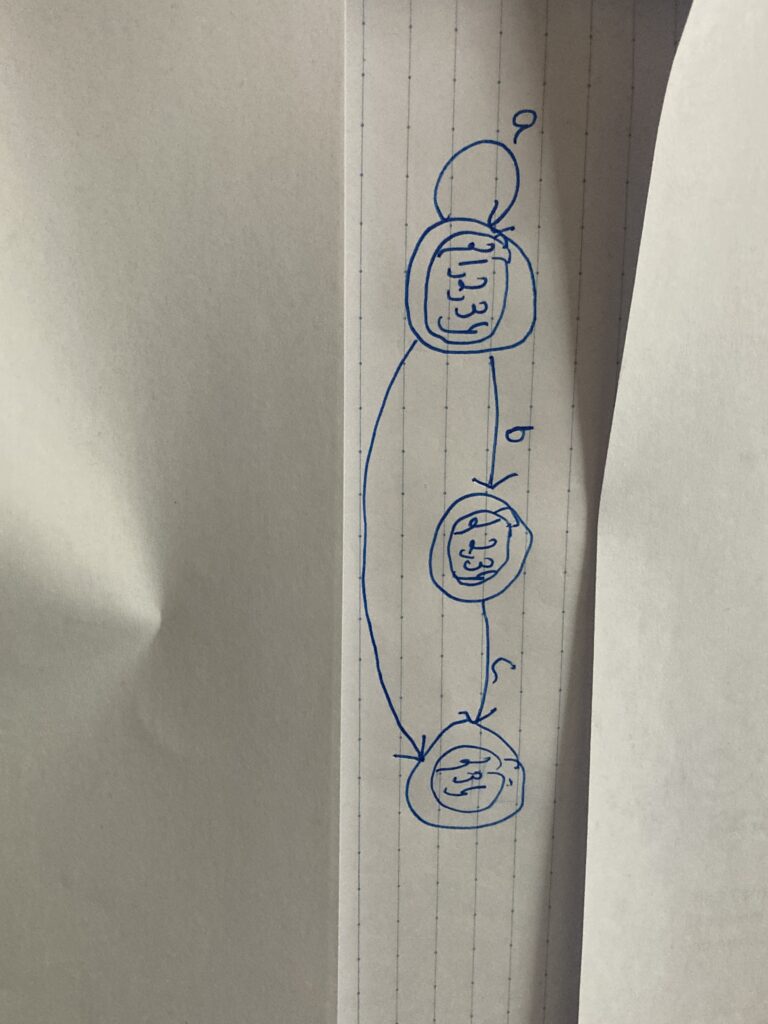
Once we have these three special vertices we can define \mathcal{M}' along with the set V(\mathcal{M})={W\subseteq V(M)|W=\overline{W}}. In essence this gives us that the states (or vertices) of \mathcal{M}' will be precisely these three special vertices. Instead of the term special we will use ‘accept’ vertices and formally define W as accept if it contains an accept vertex of \mathcal{M}. Well we have the vertices… what about the edges?

We define another set W_S={c\in V(M)} with the condition that you can reach v in a single S-arrow from a vertex in W. It follows that our edges will be defined by (w, \overline{w_s}) where w\in W and w_s\in W_s. This generates the following picture.

Edge labeled FSA

Step 2: Obtaining the DFA
At this point, we are tempted to be finished, however, we do not yet have our complete DFA. This picture shows an automaton with the start state having an edge of each element in S (the entire alphabet) and each vertex is connected by a labelled edge and is an accept vertex. Moreover, we define the state connected to edges of all elements as the unique start state. However, looking back on the definition of a complete DFA we are only part of the way there. We must have every vertex in our graph to have an edge leaving it, labelled by each element of S.

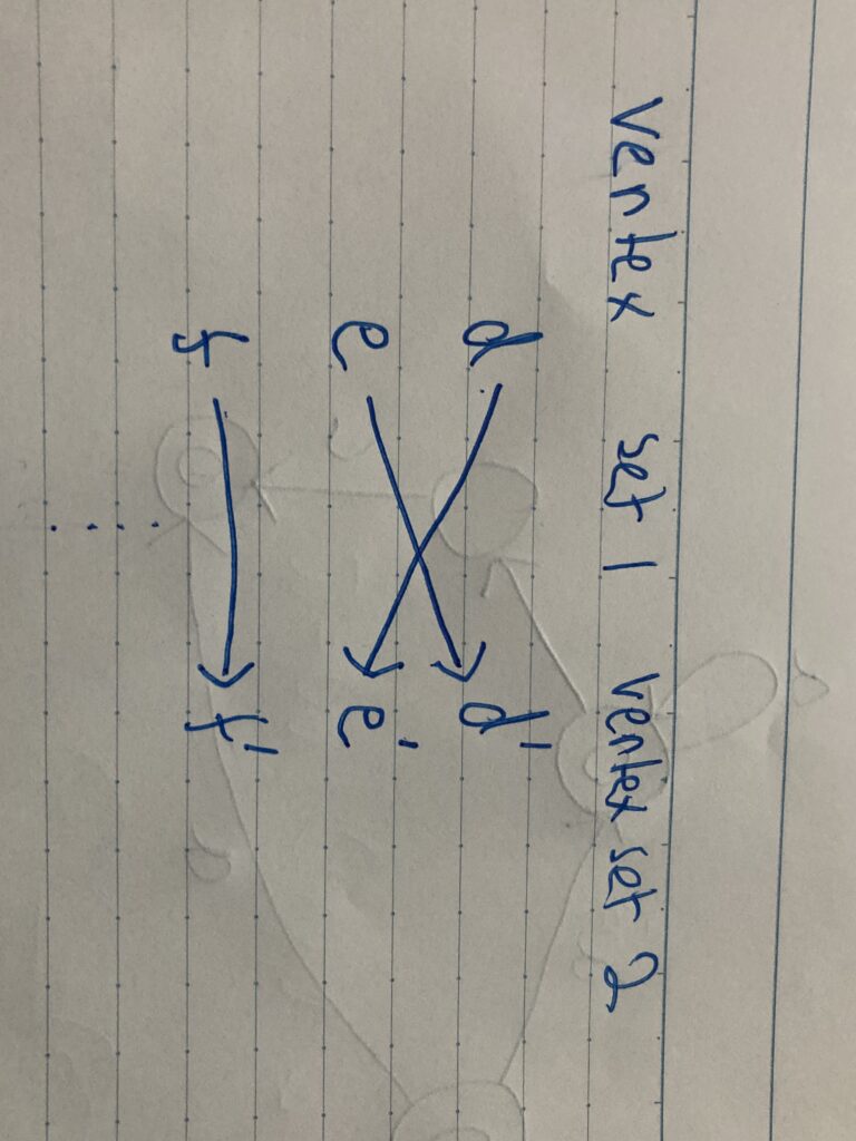
We thus must extend our process by taking \mathcal{M}' as an FSA, which it certainly is, and will map it to \mathcal{M}'' which will be an automaton adhering to all necessities of a DFA. We take V(\mathcal{M}'')={W\subseteq V(M')}. We will draw an edge with labels from S of the form (w,w') for w\in W and w'\in W' under the condition that for all vertices v\in W there exists v'\in W' such that (v,v') is an edge labelled by S and for all v'\in W' there exits a v\in W where (v,v') is also labelled. This creates the surjective mapping and completes our claim that a language on FSA is accepted by a DFA as well. This is illustrated below by the two vertex sets mapping to each other surjectively which is what we manifest in step 2.

Surjective mapping of vertices

Our theorem, however, is to show that the DFA must be complete. This can be simply demonstrated by finding that any FSA can be transformed into a complete FSA by adding a dead vertex to the automaton. This process is demonstrated below by an automaton on S={a,b} where the dead vertex is labelled D on the right of the figure. We notice that in order to keep the process finite and avoid adding dead states forever, we draw edges that loop back to the dead vertex and thus conclude the process of transitioning the FSA to a complete FSA.
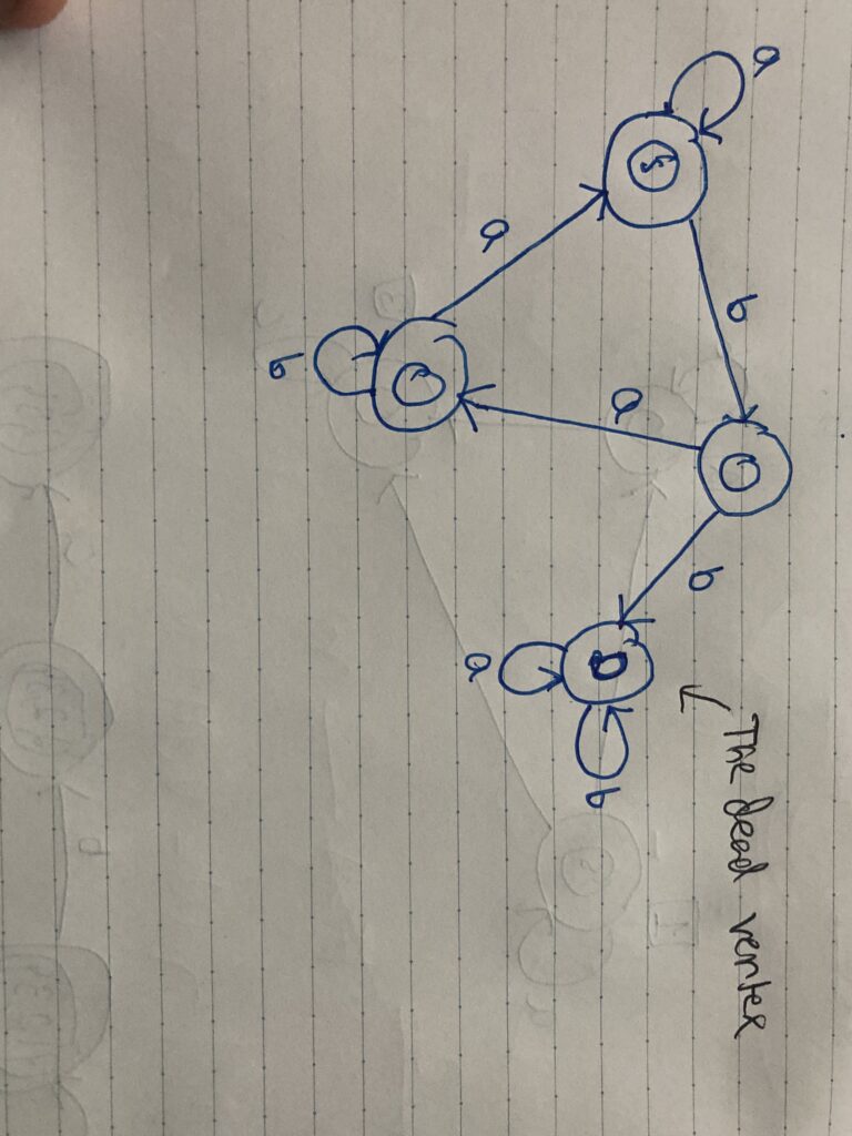
Dead vertex example

We concluded class with a definition about regular languages.
Definition 4:
The language \mathcal{L} is a regular language if there exists an FSA whose corresponding language is \mathcal{L}.

This will lead to a theorem about languages which are accepted by non-deterministic finite state automata corresponding to the languages accepted by the set of regular languages. Furthermore, this begs the question of whether all languages are regular. We can also ponder how this will all connect to normal forms and last class’ content.

Posted in Uncategorized | 4 Comments

Week 5 Monday : Serre’s Property FA and Normal Forms

Serre’s Property FA

Welcome to Week 5! I can believe we’re halfway done with this class! We ended Wednesday’s class on free products with a claim : if H \leq A*B and H is finite, then H is conjugate to a subgroup of A or B.

It turns out that this is actually a corollary of a much more general statement, albeit one that at first sight appears to be talking about something completely separate. We want to show that every finite group under any action on any tree has a universal fixed point. I’ll provide a somewhat sketchy proof below; you’ll see that it learns heavily on the finiteness of the group.

Pick an arbitrary tree and an arbitrary action. Let’s now pick an arbitrary vertex and look at the orbit of that vertex under that action. Since our group is finite, this orbit will be finite too. Let T' be the subtree spanned by the orbit of this vertex. Since our orbit is finite, this subtree will be too! So then G acts on T'. Note that it will act on the vertices in our orbit, but the intermediate vertices will be acted on as well because there is a unique path between two vertices, so under the action this path must be preserved, so these intermediate points all must be translated too. This action preserves degree! This allows us to ‘prune’ the leaves (vertices with degree one). If we continually prune this subtree, we are left with two cases.

our two cases after excessive pruning. (sorry tree!)

In the first case, if it acts on a singular vertex, this action must be the trivial action! In the other case, either one of the vertices is the fixed vertex or the midpoint of the edge is a the fixed vertex. Boom.

This property — that every action by a group G on any tree leaves a global fixed point — is called Serre’s Property Fixe Arbre (Property FA) for short. Now back to our original claim : if H \leq A*B and H is finite, then H is conjugate to a subgroup of A or B. We have shown that every finite group has Property FA, so let us consider a tree A*B acts on: the Bass-Serre tree! Recall that stabilizers of edges of the Bass-Serre tree are trivial, so the only case is that the universal fixed point can be a vertex, whose stabilizer is conjugate to A or B in our Bass-Serre tree. Boom.

This is where we say goodbye to free groups (at least as one of our primary objects of study), so I’ll state some cool theorems about Property FA (without proof, check out section 3.10 in Groups, Graphs, and Trees for proofs).


If G has Property FA, then any quotient of G also has Property FA.


For n \geq 3 GL_n(\mathbb{Z}) has Property FA.

The automorphism group of a free group \mathbb{F}_n where n\geq 3 has Property FA.

I think it’s cool to think about the automorphism group of a free group because first of all it’s an example of an infinite group (this group is huge!) with property FA and also it highlights another link free groups have with linear algebra! Jakob Nielsen showed that the automorphism group of the free group with basis x_1,x_2,\dots ,x_n is generated by the 4 elementary Nielsen transformations which are

  1. swapping two generators
  2. cyclically permuting the whole set of generators
  3. replacing a generator with its inverse
  4. replacing a generator x_1 with x_1x_2

    These 4 transformations correspond to the elementary row operations! The first two are the operations of switching any rows you’d like. The third is scaling a row by an invertible scalar, and the fourth corresponds to adding rows.

Normal Forms

We now switch our focus to the word problem, except this time more in depth. To do so we introduce some vocabulary and review some notions from before. Let’s start with an example we’re familiar with : a presentation for D_{10} = \langle a,b | a^2=b^5=e, aba^{-1} = b^{-1} \rangle. Take a look at two elements on this generating set, aba^{-1} and b^{-1}. According to our presentation, these elements should refer to the same thing, but they’re spelled differently. This is exactly to do with the word problem – it’s a question of how we define these equivalence classes.

Let’s take a step back. Take a generating set S, our alphabet and consider the free monoid S^* which is words over our alphabet, containing formal inverses. Note the subtlety — S^* contains formal inverses hinting at the fact that we’ll later want to consider this as a group, but we haven’t put any relations in place between these formal inverses yet! Then, there is a natural transformation \pi : S^* \rightarrow G. Note that placing this group structure gives meaning to elements in our free monoid, but our problem with the mispellings of the same still has not been solved.

Ideally, we’d like one clean representative on our alphabet per element of our group G. This is exactly the idea of a normal form. It is a choice of name for each element in G. More formally, it is a function \eta : G \rightarrow S^* such that \pi \eta =id.

Let’s look at a few examples.

Our old friend the free group G = \langle a,b | \rangle

The most logical normal form might be freely reduced words, but another possible normal form (courtesy of Horace) is \{waa^{-1}\} where w is freely reduced. This example highlights the fact that a normal form is a choice! Even though this is a super weird choice, it is still a normal form.

Let’s now look at \mathbb{Z} \times \mathbb{Z} : \langle s,t | st = ts \rangle

Here, we get a ton of different options. We can move all of one generator to the front, or the other, or some mix.

NF_1 = \{ t^xs^y|x,y \in \mathbb{Z} \}

NF_2 = \{ s^xt^y|x,y \in \mathbb{Z} \}

NF_3 = \{ (st)^xt^y|x,y \in \mathbb{Z} \}

Since we’re more comfortable with \mathbb{Z} \times \mathbb{Z}, let’s pick a word on our alphabet, say stsststt look at the normal forms on our Cayley graph.
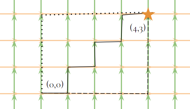
our three normal forms visualized

Taking the green arrows to be our generator t and the orange to be our generator s, we can see that normal forms correspond to picking paths to elements in our Cayley graph! Under NF_1, our word looks like t^3s^4 and in the graph, this means go all the way up, then all the way right. Under NF_2, it is s^4t^3, that is, go all the way right, then all the way up. Finally, our funkiest one NF_3 makes our word (st)^3t, which says take steps up, then go all the way right.

We also talked about normal forms that were ‘combings’, that is any path to an element that is already on a larger path to a different element is also a normal form. In other words there are no annoying knots (backtracks for example) when we choose an element on a path and inspect its normal form.

The idea of normal forms transforms our word problem — we ask if given a word on our generators, can we find the normal form for this word in a finite amount of time? As Sam pointed out, this is really just transferring of our algorithm.

Next class we’ll build up some more vocabulary to talk more concretely about the word problem and machines we’ll build to potentially solve it. Thank you for reading!

Posted in Uncategorized | 4 Comments

The Mystery of a Presentation of BS(1,2)

On Friday, Professor Alden Walker gave a lovely talk on the Baumslag-Solitar Groups. I was fascinated by the Cayley graph of BS(1,2). Also, he discussed geodesics between group elements (a shortest but not necessarily unique! path in its Cayley graph that travels one from another). The nice presentation (the focus of this post) of BS(1,2) gives a very easy way of identifying geodesics so that we can even say a bit more about the spheres (the number of group elements a certain geodesic length away from a fixed element), which indeed involves his own research!

With the above said, BS(1,n) is a very special group bearing many interesting properties. In this blog post, I will highlight some special features of the action of BS(1,n) on \mathbb{R}. This action is very different from the actions we used to see in the past three weeks, specifically reflection actions. Without further due, let me recall the definition of BS(1,n).

In the following definition of BS(1,n), we directly view them as a subgroup of Homeo(\mathbb{R}) so that the aspect of them as actions is straightforward. Like what Professor Walker discussed, given the vastness of Homeo(\mathbb{R}), we would like to find a subgroup that is not trivial, but also not too completely so that any concrete understanding is beyond our ability.

Definition 1. Note that a(x)=nx, where n\geq 2 \in \mathbb{Z}, and b(x)=x+1 are elements of Homeo(\mathbb{R}). Then, we say that the Baumslag-Solitar Group BS(1,n) is the subgroup of Homeo(\mathbb{R}) generated by a(x)=nx and b(x)=x+1.

Then, we directly state a fact regarding BS(1,2).

Fact: BS(1,2)=\langle a,b\mid ab=b^2a \rangle.

Utilizing the above presentation of BS(1,2), we draw the Cayley graph of BS(1,2).

Diagram 1. A plane of the Cayley graph of BS(1,2). *From Wikipedia, Baumslag–Solitar group.

In the above diagram, we see the relator ab=b^2a of the generating set gives each rectangle, in which we can either go red twice and blue once or go blue once and red once. In other words, this diagram manifests the “weird commutativeness” of BS(1,2). However, Diagram 1 is only part of the story since we are missing a red edge. Indeed, adding another red edge would result in generating another plane. Therefore, we form a “3-dimensional” picture of the Cayley graph.

Diagram 2. The Cayley graph of BS(1,2) given by the default generating set. *From Wikipedia, Baumslag–Solitar group.

I know you will be amazed by the nice animation above! Thank you, Wikipedia! Clearly illustrated by the animation, we extend another copy of the plane whenever we introduce another red edge “skew” from the current plane.

After introducing BS(1,2) rigorously, I discuss some “weridness” of BS(1,2) \curvearrowright \mathbb{R}. For the linear function a(x)=2x, it achieves the effect of “stretching” the real line. For the linear function b(x)=x+1, we achieve the effect of translating the real line by a unit length. Combining two together, we are able to translate the real line to an arbitrarily small distance. Wait a minute, isn’t that strange? This means that the action is no longer “discrete” but extremely “continuous”.

We can make the idea of an action being discrete a bit more rigorous.

Definition 2. An action G\curvearrowright X is called discrete if every orbit form a discrete subset of X. In other words, for every x\in X, there exists a neighborhood N_x of X such that the intersection of the orbit of x and N_x is exactly x.

Notice that the reflection group D_\infty \curvearrowright \mathbb{R} with reflections an unit distance apart is discrete, which agrees with our intuition that symmetries generated by reflections are rigid and discrete. First, we note that a fundamental domain of D_\infty  \curvearrowright \mathbb{R} is [0,1]. From there, we conclude that the orbit of a point is \{2n\pm r \mid n\in \mathbb{N}\}, where r is the decimal value of x. Therefore, we can definitely find a small enough neighborhood such that the intersection is exactly x.

However, when we go back to BS(1,2) \curvearrowright \mathbb{R}, it is a completely different story. Let’s consider the point 0, its orbit includes all points 1/2^k since

    \[a^{-k}b(0)=\frac{1}{2^k}.\]

Thus, no matter how close we choose a neighborhood around 0, it would necessarily intersect with some point in the orbit other than 0. Therefore, this action is not discrete.

Another difference we can make between BS(1,2) \curvearrowright \mathbb{R} and D_\infty \curvearrowright \mathbb{R} is the cardinality of the stabilizer. Often times, we would think that the stabilizer of a point is finite, just like in the case of D_\infty \curvearrowright \mathbb{R}. However, it is far from being true for BS(1,2) \curvearrowright \mathbb{R}.

Definition 3. An action G\curvearrowright X is called proper if the stabilizer of any point x\in X is finite.

For BS(1,2) \curvearrowright \mathbb{R}, we claim that the stabilizer is infinite since \langle a \rangle (elements are scalar functions) would keep 0 fixed. Therefore, the action of BS(1,2) on the real line is neither discrete nor proper. Indeed, similar arguments can be applied on any BS(1,n) so that the action of BS(1,n) on the real line is neither discrete nor proper!

Following the “weridness” of BS(1,2) \curvearrowright \mathbb{R}, can we categorize the orbits of any given points? The answer is yes, and is implied from the following proposition.

Proposition 4. The elements of BS(1,2) are the linear functions g:\mathbb{R} \to \mathbb{R} are in the form

    \[g(x)=2^n\cdot x + \frac{m}{2^k},\]

where n,m,k are all integers.

I sketch a proof of the above proposition. First, we note that the elements of BS(1,2) are all linear functions since composition of linear functions are linear. Then, we use induction on the length of words. For the length 1 case, we note that the formula holds for all a,a^{-1},b,b^{-1}. Assume that the formula holds for all length \leq N-1. Then, we look at the first word. Indeed, there are only four possibilities a,a^{-1},b,b^{-1} again. No matter which one we consider, composing it with the rest (length N-1 now so that we can use the hypothesis) would again yield the form mention in Proposition 4. Therefore, the statement follows.

As a final remark in this post, the above proposition can be proved for any BS(1,n) with similar lines of arguments. You can give yourself a small challenge to supply a proof to yourself!

Posted in Uncategorized | 7 Comments

Week Four Wednesday: Free Products and Word Metrics

[At the beginning of class, we discussed possible topics for the final project – for more information, click the ‘Course Info’ link at the top of the page. We also looked at some very nice drawings of Bass-Serre trees.]

We started out today’s lesson by continuing our discussion of free products. Here are a couple neat facts about free products of groups:

1. Free products of groups are free if and only if both original groups are free. Proving this will be a problem on the upcoming problem set.

2. Let A and B be groups. Let C = \{[a,b] | a \in A, b \in B \} - \{e\}. Then any subset of C is a basis for a free subgroup of A*B. A complete proof of this claim is fiddly and annoying [see: the latter half of this post].

Let’s switch gears for a moment.

Definition: A metric on a space S is a function d: S \times S \rightarrow \mathbb{R}_{\geq 0} such that
1. The distance from a point to itself is 0. That is, d(x,x) = 0 for any x \in S.
2. d is symmetric; in other words, d(x,y) = d(y,x) for every x,y \in S.
3. d obeys the triangle inequality. This means that for any x,y,z \in S, d(x,y) + d(y,z) \geq d(x,z).

A space equipped with a metric is called a metric space. Why does this help us study the geometry of groups? To answer this question, we need to define the following notion:

Definition: If g is in a group G generated by a set S, the word length |g|_S is the minimum length of a word on S that represents g.

Note that the length of an individual word may be different from the word length of the corresponding group element. For example, if G is a group with generating set S = \{a,b \}, then the word length |a^5 b^{2} b^{-2} a| = 6.

This brings us to the following definition:

Definition: Let G be a group with a generating set S. The word metric on G with respect to S is a function d: G \rightarrow \mathbb{R}_{\geq 0} such that d(g,h) = |g^{-1}h|_S.

One thing that helps me visualize a word metric is to consider the Cayley graph \Gamma of G with respect to S. Recall that if g,h \in G, then g^{-1}h is expressed by the sequence of edges in the path from g to h in \Gamma. This means that if d is the word metric on G with respect to S, then d(g,h) is the length of the shortest path from g to h in \Gamma. This lends a nice geometric interpretation to the concept.

Note that different generating sets for G may yield completely different word metrics. For instance, if you use the entire group as a generating set, any two elements will have distance 1 under the word metric. This is not true in general.

Here are a couple examples of word metrics in action:
1. If G = \mathbb{Z} and S = \{1\}, then the word metric d(g,h) is given by |h-g|.
2. If w_1 and w_2 are words, let pref(w_1,w_2) denote the longest common prefix of w_1 and w_2. If G is a free group generated by S, containing freely reduced words w_1 and w_2, then d(w_1,w_2) is given by |w_1|_S + |w_2|_S - 2\cdot pref(w_1,w_2).
3. The word distance from any group element g to the identity is the length of the shortest word expressing g over the generating set.

Now that we know a bit about word metrics, we can switch back to our discussion of free products:

Theorem: If A and B are finite groups then, A*B is virtually free.

[Recall from last class that a group is virtually P (for some property P) if it contains a finite-indexed subgroup that is P.]

Proof. Let \phi : A*B \rightarrow A \times B be a homomorphism defined as follows: for any element a in the generating set of A, \phi(a) = a. For any element b in the generating set of B, \phi(b) =b.

[Side note about notation: the presentation we are using for A \times B is \langle A \cup B | ab = ba, a \in A, b \in B \rangle. An element a in this generating set can be written in more set-theoretic notation as (a, id_B) \in A \times B. Similarly, a generator b can be written as (id_A, b). So, we can also think of \phi as mapping a to (a,id_B) and b to (id_a,b) for any a \in A and b \in B.]

Observe that every generator of A \times B is mapped to by a generator of A * B. This implies that im\phi = A \times B. By the First Isomorphism Theorem, A * B /ker\phi \cong A \times B. Because A and B are finite by assumption, [A * B :ker\phi] = |A \times B| < \infty. Therefore, ker\phi is a finite-indexed subgroup of A*B. Let’s try showing ker\phi is free.

There are a few ways we can go about this:
1. We can find a basis for ker\phi.
2. We can show ker\phi acts freely on a tree.
3. We can use the ping-pong lemma.

We will be using the first technique. I’ll assert that a basis for ker\phi is given by C = \{ [a,b] | a \in A, b \in B \} - \{ e \}.

Claim: C generates ker\phi (left as an exercise to the reader).

Claim: Any reduced word on C is non-trivial in A * B. We’ll prove this inductively on the length of the word.

Inductive hypothesis: every reduced word w such that |w|_{C}  = \ell satisfies the condition that |w|_{*} \geq \ell + 3.

[Here, |w|_{*} denotes the syllable length of w with respect to the groups A and B. Recall that the syllable length of w is the number of ‘runs’ in w, where a run is a maximal subword consisting entirely of letters from a single one of the original groups. For example, the syllable length of a_1 a_2 a_3 b_1 a_4 b_2 a_5 a_6 is 5. Any letter in C can be expressed as aba^{-1}b^{-1} for a \in A and b \in B. So, if w = c = aba^{-1}b^{-1}, then |w|_{*} = 4.]

Base case: |w|_{C} = 1. Then w \in C, so w = aba^{-1}b^{-1} for some a \in A and b \in B. Therefore, |w|_{*} \geq 4 = 1 + 3 = \ell + 3.

Inductive step: Let w be a word such that |w|_C = \ell + 1. Therefore w = c_1 c_2 ... c_{\ell} c_{\ell + 1} where c_i \in C. Consider the word w' = c_1 c_2 ... c_{\ell}. By the inductive hypothesis, |w'|_{*} \geq \ell + 3.

Observe that each letter c_i in w can be expressed as a_i b_i a_i^{-1}b_i^{-1} for some a_i \in A and b_i \in B. Assume without loss of generality that the second to last syllable of w' is from A and the last syllable is from B. So, we have that:

w = x_1 x_2 ... x_k a_{\ell} b_{\ell} c_{\ell + 1} where every x_i \in A \cup B.

Case 1: c_{\ell + 1} = [a,b]. In other words, there exist a \in A and b \in B such that c_{\ell +1} = aba^{-1}b^{-1}. Therefore, we can express w as:

w = x_1 x_2 ... x_k a_{\ell} b_{\ell} a_{\ell +1} b_{\ell +1} a_{\ell +1}^{-1}b_{\ell +1}^{-1}. This word cannot be reduced further, as we have no relators between the elements of A and B. Thus, we have that this word has four more syllables than w', so

|w|_{*} = |w'|_{*} + 4 \geq \ell + 3 + 4 > (\ell+1) + 3.

Case 2: c_{\ell + 1} = [a,b]^{-1} for a \in A and b \in B (recall that the inverse of an element of a set can be included in words over that set). We have that:

w = x_1 x_2 ... x_k a_{\ell} b_{\ell} b_{\ell +1}^{-1}a_{\ell +1}^{-1}b_{\ell +1}a_{\ell +1}. There are two subcases:

i) If b_{\ell} \neq b_{\ell + 1}, then the word is freely reduced as is, and we have that |w|_{*} = |w'|_{*} + 3 \geq \ell + 3 + 4 > (\ell + 1) + 3.

ii) If b_{\ell} = b_{\ell + 1}^{-1}, then b_{\ell} b_{\ell +1} cancels to e, and we have that w = x_1 x_2 ... x_k a_{\ell} a_{\ell +1}b_{\ell +1}^{-1}a_{\ell +1}^{-1}. I claim this word is reduced. Note that if a_{\ell} and a_{\ell +1}^{-1} cancel, then (a_{\ell} = a_{\ell+1}. This implies c_{\ell} = a_{\ell}^{-1} b_{\ell}^{-1} a_{\ell} b_{\ell} = (b_{\ell}^{-1} a_{\ell}^{-1} b_{\ell} a_{\ell})^{-1} = c_{\ell}^{-1}, which implies w is not reduced over C.

So, we have that |w|_{*} = |w'|_{*} -1 + 2 \geq \ell + 3 -1 + 2 = (\ell + 1) + 3. This concludes the inductive argument.

Thus, any reduced word on C is non-trivial in A * B. Because C also generates ker\phi, C is a basis for ker\phi. This implies ker\phi is a free subgroup of A*B. Because we showed above that ker\phi has finite index in A*B, A*B is virtually free.

This concludes the proof.

Looking ahead: On Friday, we’ll have a guest lecture on Baumslag-Solitar groups. On Monday, we’ll prove the following theorem:

Theorem: If a finite group acts on a tree, there is a universal point fixed by every element of the group.

I want to conclude this blog post by discussing a random fact I only know for bizarre coincidental reasons: word metrics are really hard to compute. While an individual group may permit an efficient algorithm to compute the distance between two of its elements, trying to compute a word metric on a class of groups is usually quite hard. This often remains true even when the class is quite restricted.

To see what I mean, consider the following problem: given a symmetric group S_n, a generating set T of transpositions, and two elements g, h \in S_n, what is the shortest word on T needed to express g^{-1}h?

Even this problem, which deals only with order two generators over a very restricted class of finite groups, is known to be NP-hard [1], providing strong evidence there is no efficient algorithm to solve it. The problem only becomes harder if one makes it more general.

[1] Miltzow, L. Narins, Y. Okamoto, G. Rote, A. Thomas, and T. Uno, “Approximation and hardness for token swapping,” Proceedings from the 24th Annual European Symposium on Algorithms, 2016. arxiv preprint here: https://arxiv.org/abs/1602.05150

Posted in Uncategorized | Tagged , | 6 Comments

Week 4 Monday: The Free Product of Groups

Today we discussed a new way to combine two groups: the Free Product, and looked at the Cayley Graph of such products which led us to discuss Bass-Serre Trees.

The Free Product of Groups

Definition. Let A and B be groups. The free product A \ast B is the group whose underlying set is

\{a_1 b_1 a_2 b_2 \dots a_n b_n\, | \, a_i \in A-\{e\} \text{ for } i\ne 1, b_i \in B-\{e\} \text{ for } i \ne n, a_1 \in A, b_n \in B\}.

With the operation of concatenation along with free reduction and “glomming” of elements of the same starting group.

Essentially, we are alternating elements of A with elements of B, allowing for the possibility of starting with either an a or a b and ending with either an a or a b. This definition looks very similar to the definition of the free group on two elements. One key difference, however, is the lack of exponents on the letters in the words (in the definition). This arises from the fact that in F_2, we are creating words on a generating set and in A \ast B we are creating words on the entire underlying set.

Like free groups, our group operation is concatenation, but with a small twist. Our underlying set is not actually the words themselves, but the equivalence classes represented by the words. This ensures that we continue to stay within the group after concatenation. We also continue to allow for free reduction, similar to free groups. Finally, we don’t want two elements of the same group right next to each other. Instead, we determine the value of their product within the group and use that element instead. This allows us to continue following the notation set out above.

Let us now consider what the presentation of A \ast B looks like. Let A = \langle S\,|R\,\rangle and B = \langle T\, | \, Q\rangle. Then,

A \ast B = \langle S \amalg T\,|\, R \cup Q\rangle.

The \amalg symbol represents the disjoint union of S and T. This means that we have to name the elements of S and T such that they share no elements in common. The relators are the words that are equivalent to the identity under the group operation. These don’t change when we add more generators, so the relators of A \ast B are simply all of the relators of A and all of the relators of B. One might ask, are there any relators which combine both elements of A and elements of B? The answer is no, we do not allow any relators which we do not already have and since we have a disjoint union of the elements, no relators combine elements of A with elements of B.

Since we can have words of any length and there is no mechanism for a word containing a’s and b’s to be the identity unless it is trivial, it naturally follows that A \ast B is infinite unless at least one of A and B is trivial and the other one is finite. For example, if we take \mathbb{Z}/2\mathbb{Z} \ast \mathbb{Z}/2\mathbb{Z} we get \langle a,b\, | \, a^2=b^2=e\rangle, which is D_\infty, or the infinite reflection group. Even though \mathbb{Z}/2\mathbb{Z} is about as finite as we can get, and we are starring it with itself, we still get an infinite group.

Another example of free products if \mathbb{Z} \ast \mathbb{Z} = \langle a,b\,|\rangle = F_2. More generally, F_n \ast F_m = F_{n+m} since we just combine the two lists of generators and continue to have no relators.

Cayley Graphs of Free Products

Let us now consider the Cayley graph generated by one of these free products. Consider \mathbb{Z}/3\mathbb{Z} \ast \mathbb{Z}/2\mathbb{Z} = \langle a^3=b^2=e\rangle. The Cayley Graph is shown below.

This Cayley graph alternates triangles (three-cycles) with undirected edges representing the \mathbb{Z}/3\mathbb{Z} and \mathbb{Z}/2\mathbb{Z} nature of the group, respectively. Similarly, for \mathbb{Z}/3\mathbb{Z}/ \ast \mathbb{Z}/5\mathbb{Z}/ = \langle a^3=b^5=e we get:

This graph consists of alternating triangles and pentagons. If we squint, close one eye, and spin around, this graph kind of looks like a tree. In fact, we can build a tree out of it called the Bass-Serre Tree (see below).

To construct the Bass-Serre Tree we place vertices on the inside of each of the triangles and pentagons and connect them through the vertices of the original Cayley graph. We label the new vertices with cosets of our two original groups and the new edges with the vertices they passed through.

Final Facts and Theorems

Finally, we stated and, in some cases, proved two statements about biregular trees and free products.

Theorem. A \ast B acts on a biregular tree such that the fundamental domain of the action is two vertices with a single edge connecting them where the stabilizers of the vertices are conjugates of factor groups and stabilizers of edges are trivial.

Corollary. If G acts on a biregular tree such that there exist subgroups of G, A and B, so that the fundamental domain of the action is two vertices with a single edge connecting them where the stabilizers of the vertices are conjugates of factor groups and stabilizers of edges are trivial, then G \cong A \ast B

We also briefly discussed the free product with amalgamation, but due to space and time limitations and I will not go into that here.

Lastly, we defined virtually and introduced a theorem that we will prove next time:

Definition. A group G is virtually P if there exists a finite index subgroup H \le G such that H has the property P.

Theorem. If A and B are finite, then A \ast B is virtually free.

Resources Used:

Free product of groups. Encyclopedia of Mathematics. URL: http://encyclopediaofmath.org/index.php?title=Free_product_of_groups&oldid=46986

Free Product. Wikipedia. URL: https://en.wikipedia.org/wiki/Free_product

Posted in Uncategorized | 5 Comments