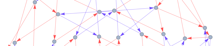
Today’s lecture was held outside, in the lovely warmth and sunlight. We considered two ways to approach the following statement.
Claim. If  , then
  is free.
A Geometric Group Theory Proof
Instead of proving this claim directly, we started with a more general statement.
Theorem. If  freely and without edge inversions, then
  is free.
Proof. Let  be a tree, and consider an action
  such that the action is free and without edge inversions. Let
  be a fundamental domain of over this action.
If  , then this intersection must consist exactly of points
  such that is the midpoint of an edge. This follows from how we construct fundamental domains and the definition of a tree.
In particular, since trees have no cycles, the fundamental domain of a tree must consist of endpoints, edges, and half-edges. If endpoints or edges were shared between two fundamental domains, then would no longer be a partition . However, if contains a half-edge, then the other half of the half-edge must belong to some multiple  , again since we’re partitioning all of . If the midpoint of the edge belonged to one or neither, we wouldn’t be able to multiply any
  to obtain the midpoint, so the midpoint must belong to exactly two fundamental domains.
We want to use these midpoints to prove that is acting freely. To that end, we’ll seek to show that  generates a (free!) basis for . Symbolically, we want to show that for
![\[S = \{g \in G \ | \ \mathcal{F} \cap g\mathcal{F} \neq \emptyset\},\]](https://ggt.math.sites.carleton.edu/wp-content/ql-cache/quicklatex.com-de1b7b6369defbb869ee7a02f5099b32_l3.png "Rendered by QuickLaTeX.com")
that  .
.
Since acts freely on , we expect any for  that
that  , and by definition of a fundamental domain for an action, we expect for
  and
and  that
that  . Therefore every
  satisfies
  , and so contains all of .
We additionally seek to show that no freely-reduced non-trivial word  is trivial in . Toward that goal, consider some midpoint on our tree, an arbitrary
  . We may consider the path generated by “building up” to
  , or more precisely, the sequence of vertices generated by




With these midpoints on our tree in mind, we can consider the unique reduced path generated by connecting  to
to  , to
, to  , and so on. We’ll name these paths
  , and so on. Trees have pretty rigid structure; we can take advantage of this structure in order to make some pretty rigorous statements about each
  . Toward a contradiction, suppose that we have a loop, or more precisely that the same
  occurs more than once in the path from to
  . Since is a tree and thus contains no cycles, the loop implies we must have backtracked:
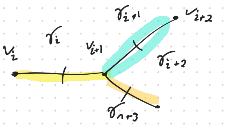
But we see that a backtrack implies that three separate fundamental domains all shared the same midpoint edge; this contradicts the definition of an edge midpoint. Instead, it must be the case that every non-trivial word in corresponds to a non-trivial action. Thus we know that freely-reduced non-trivial words in are non-trivial on , and so is indeed a basis of , and since our basis includes no relators, is free. 
Our original claim, that subgroups of free groups are themselves free, follows as a corollary. In particular, if is free and  , then and both act freely on the Cayley graph of . Since acts freely, is free. .
A Topological Proof
For the second part of the lecture, we considered a topological proof of our original claim that subgroups of free groups are free.
Definition. Given a space  and a point
  , a fundamental group
  is the group formed by the equivalence class of loops that start at
  over the operation of concatenation.
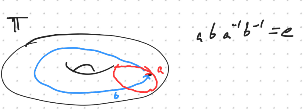
Example. Consider the torus  , and some point
  . We have (at least) two loops, one given by the vertical circle in red, and one given by the horizontal circle in blue:
Fact. For any graph  , it’s the case that
  is free.
I have very little background in topology, but I think this relates to the idea of thinking of free groups as little “bouquets” of loops. In some sense, I suspect this is what it means to be a free group.
Definition. Let and  be spaces, with a map
![\[f: Y \to X\]](https://ggt.math.sites.carleton.edu/wp-content/ql-cache/quicklatex.com-90681cb8a1e148d28e4550b7e0492f58_l3.png "Rendered by QuickLaTeX.com")
such that  is continuous, surjective, and locally homeomorphic. Then covers, or is a cover of, the space .
Fact. For some spaces  where is a cover of ,
  satisfies
  , and every
  corresponds to an open cover of . This property is known as Galois Correspondence.
We can use this assortment of facts and definitions to show that subgroups of free groups are free. For some , it’s the case that  . By Galois Correspondence, we know that any implies is a cover of , and so must be free.
 is the unique froups os that for any
  such that the diagram below commutes.
 .
. if and only if
  . I won’t spoil the puzzle for anyone who’s working on it but for a slightly cryptic hint you can read the following sentence backwards: STNEMELE HCUS GNINIAMER EHT YB TUO DOM.
 if and only if
  .
. the element
 ![[a,b] := aba^{-1}b^{-1}](https://ggt.math.sites.carleton.edu/wp-content/ql-cache/quicklatex.com-d53509a1d1250548efd99d1cb45b385d_l3.png "Rendered by QuickLaTeX.com") is called a commutator. The subgroup of G generated by the set of commutators is called the commutator subgroup and is denoted
is called a commutator. The subgroup of G generated by the set of commutators is called the commutator subgroup and is denoted ![[G:G] \in G](https://ggt.math.sites.carleton.edu/wp-content/ql-cache/quicklatex.com-5ba2004fef28ce606670c968fa5c2898_l3.png "Rendered by QuickLaTeX.com") . To see that this subgroup is normal, let
. To see that this subgroup is normal, let ![c_1 \ldots c_n \in [G:G]](https://ggt.math.sites.carleton.edu/wp-content/ql-cache/quicklatex.com-373911dd1293c5a6f4a45792485abfe6_l3.png "Rendered by QuickLaTeX.com") , where the
, where the  are commutators. We must show that for all
 ![g c_1 \ldots c_n g^{-1} = g c_1 g^{-1} g c_2 g^{-1} \ldots g c_n g^{-1} \in [G:G]](https://ggt.math.sites.carleton.edu/wp-content/ql-cache/quicklatex.com-b40816c00f5795d1508382f26f1a03b1_l3.png "Rendered by QuickLaTeX.com") . To do so we need only show
. To do so we need only show ![gc_ig^{-1} = g [a,b]g^{-1} \in [G:G]](https://ggt.math.sites.carleton.edu/wp-content/ql-cache/quicklatex.com-958683a7cbff91d3e1ab7fe4183c99a3_l3.png "Rendered by QuickLaTeX.com") which we can do by writing this element as a product of commutators:
which we can do by writing this element as a product of commutators: ![g [a,b]g^{-1} = [ga, b] [b, gb]](https://ggt.math.sites.carleton.edu/wp-content/ql-cache/quicklatex.com-ec0c821654043d0a16c11f38217da9f5_l3.png "Rendered by QuickLaTeX.com") . The resulting group
. The resulting group ![\overline{G} := G / [G:G]](https://ggt.math.sites.carleton.edu/wp-content/ql-cache/quicklatex.com-8519bd26cff8a587fdc672250e04dc8e_l3.png "Rendered by QuickLaTeX.com") is called the ablianization of
is called the ablianization of  , there exists a bijection between
  . For the harder direction, we note that taking if
  , and those are much easier to understand. Namely,
![\[ \overline{F_S} = \mathbb{Z}^{|S|}. \]](https://ggt.math.sites.carleton.edu/wp-content/ql-cache/quicklatex.com-8bd5e733baa22010177caaa402f11a79_l3.png "Rendered by QuickLaTeX.com")
 . Which is only true if
  contains an isomorphic copy of
  . Performing successive mods of these subgroups will reduce
  steps, a fact which uniquely identifies this group with the integer
  for
for  . The details are left to be sorted out.
  which is not finitely generated, namely
![\[ S = \{ a^n b a^{-n} | n \in \mathbb{Z} \} \subseteq F_2. \]](https://ggt.math.sites.carleton.edu/wp-content/ql-cache/quicklatex.com-9cd21b51b92eb9fd02fc1a61406923a7_l3.png "Rendered by QuickLaTeX.com")
 is not finitely generated, we must show that no freely reduced word in is the identity. Towards a contradiction, suppose that
 ![\[ s_1 \ldots s_n = e = (a^{k_1}b^{\pm 1}a^{-k_1})(a^{k_2}b^{\pm 1}a^{-k_2}) \ldots (a^{k_n}b^{\pm 1}a^{-k_n}). \]](https://ggt.math.sites.carleton.edu/wp-content/ql-cache/quicklatex.com-39a07b9bf44980dc534105789452ffb3_l3.png "Rendered by QuickLaTeX.com")
 and
and  which are immediately adjacent except for the powers of
  which cancel with each other, and hence must be part of an expression of the form
  which in turn looks like
  in the original word, meaning that it was not freely reduced with respect to our generating set, contradicting our assumption that there is such a freely reduced word which equals the identity. We have shown that
  , which is the free group on countably many generators.
 for every integer
  .
. , where the same idea holds in any finitely generated group. In practice this looks like using the “same” generators for the quotient group.
 then
then  acts freely on a tree
  (without edge inversion), and therefore each of its subgroups
  , but the graph
  has degree four at every vertex whereas the the graph
  has degree six at every vertex. There certainly can’t be such a tree contained as a sub-tree of
  .
.
 .
. , and let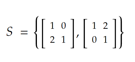

 through linear transformations. Let’s subdivide our plane into 4 sections with the lines
  and
and  and see how each element of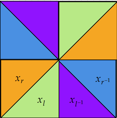
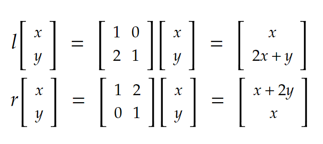
 .
.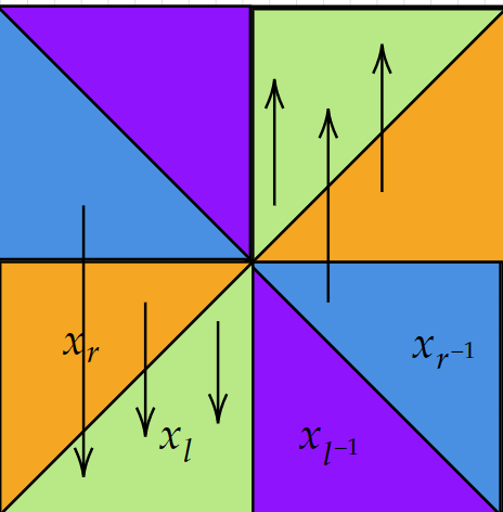
 . Everything except for
  , that is! Weird things happen with that section, and I’d encourage you guys to play around with random vectors in that section. Horace mentioned in class that it’s a good idea to look at the boundaries of our sections — this leads us to see that one boundary for
  is fixed (the one that is along the x-axis), and our other one goes to
  , which means that our new boundaries encapsulate many sections of our plane. Anyways, I think it is fine to not completely understand what happens with vectors in that area, as it is not integral to our proof. In fact, the much more important part is that every other section gets mapped into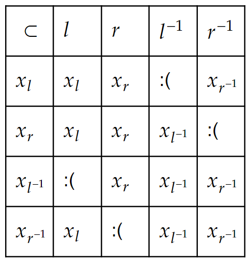
 , for some
  .
. . Let’s now pick a section of our plane for our word to act on. Since we’re given the choice, it’s important that we don’t pick our one ugly choice — that being
  , as that’s the choice that messes everything up.




 . If there exists disjoint open regions such that
  for all
  , then
  is free.
 .
.
 can be interpreted as reflections of the regular
  across a line
  in
in 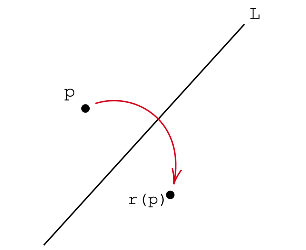
 to a point
  on the other side of
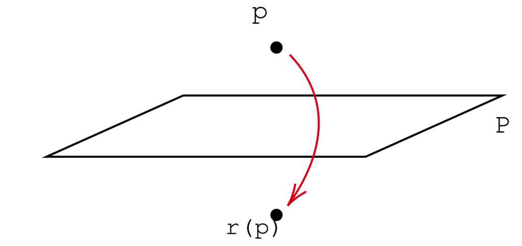
  we can consider a reflection over a plane
  :
:
 there exists a reflection across any copy of
  . Our goal for today is to look at groups generated by reflections.
 and
and  which intersect at angle
  .
.
 ?
? ,
,  ,
,  ⟷
⟷  .
. ,
,  do?
do? ⟶
⟶  about the center of the pentagon. Because we know
  , we can conclude that
 ![\[ D_{10} = \langle r,s | r^2 = s^2 = (rs)^5 = e \rangle \]](https://ggt.math.sites.carleton.edu/wp-content/ql-cache/quicklatex.com-7f29318c8ffe8fd05f85034d5a8b4763_l3.png "Rendered by QuickLaTeX.com")
 , then
  .
.  , and
, and  .
.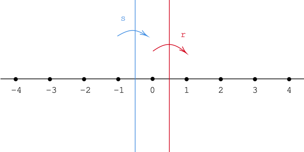
 ⟷
⟷  ,
,  ⟷
⟷  ,
,  ⟷
⟷  ,…
,… ⟷
⟷  ,…
,… and
and  . Composing
 ![\[ rs(x) = 1-(-1-x) = x+2\]](https://ggt.math.sites.carleton.edu/wp-content/ql-cache/quicklatex.com-34f477afc85f8bff9c3c619ab0191482_l3.png "Rendered by QuickLaTeX.com")
 from each other, then
  orthogonal to those lines. We call the group generated by two such reflections the infinite dihedral group, denoted
![\[D_{\infty} = \langle r,s | r^2 = s^2 = e \rangle \]](https://ggt.math.sites.carleton.edu/wp-content/ql-cache/quicklatex.com-0091c56dee0beb90c464e8e7c2904b30_l3.png "Rendered by QuickLaTeX.com")
 lies to the right of
  .
. . Let
. Let  be reflections across the planes
  ,
,  , and
, and  respectively.
 , so
, so  . This yields the following presentation of the group of symmetries of a cube:
![\[ \langle r, s, t | r^2 = s^2 = t^2 = (rs)^2 = (st)^2 = (tr)^2 \rangle \]](https://ggt.math.sites.carleton.edu/wp-content/ql-cache/quicklatex.com-161c73244696617eab989c86292950d5_l3.png "Rendered by QuickLaTeX.com")
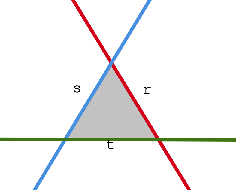
 , so
, so  . When we perform a reflection along one edge, observe that the lines along which the other edges lie are rotated. The transformations of the equilateral triangle yielded by flipping along edges can form a group. For instance, if we consider the group generated by flipping across the edges
![\[ \langle r, s, t | r^2 = s^2 = t^2 = (rs)^3 = (st)^3 = (tr)^3 \rangle \]](https://ggt.math.sites.carleton.edu/wp-content/ql-cache/quicklatex.com-8c1fbdc31286f485469d9d84fe030859_l3.png "Rendered by QuickLaTeX.com")

 is a group with a presentation of the form:
![\[W = \langle s_1, s_2, ..., s_n | s_i^2, (s_i s_j)^{m_{i,j}} \rangle \]](https://ggt.math.sites.carleton.edu/wp-content/ql-cache/quicklatex.com-c49def406731559664bb524c23b61cbf_l3.png "Rendered by QuickLaTeX.com")
 . If we say
  , we mean that there is no relation of the form
  for
for  .
. s. In other words, if
  is a relation in the presentation of a Coxeter group, there is an edge of weight
  and
and  . Note that, because
  for all
  , we don’t need to orient the edges of this graph.
 we may form the words
  , and so on. Note we are really adding in the formal inverse of everything in
  . Now we might have the feeling that these objects, namely the words on
  looks a little clumsy, we would rather see this as
  . We will say that consecutive powers of the same sign can just be summed together for notational convenience. Furthermore, if we have the construction of a group as our end goal, then we want
  to collapse to some identity element. To this end we define the empty word, which is denoted
  for all
  . We define a word to be freely reduced if it contains no sub strings
  for any
  reduces to the empty word
  if they each reduce to the same freely reduced word. We may now take the set
  , which will be the ground set of our soon to be group.
 for all
  , or any other set of cardinality
  , where the
  are integers such that
  are nonzero, and
  and
and  may be zero to allow for every possible word shape. We’ll use this group as a running example to explain the definitions and theorems to follow.
 is a set of elements that generate
  and
and  are NOT bases for
  and
and  are. Both the non examples illustrate how a non-trivial word on some basis elements can be trivial in
  , the word
  is non trivial with respect to this labelling, but when substituting to compute the value in
  . The second basis has this issue as well as the issue that it doesn’t generate
  , then
  for sets of any cardinality.
 and note that for some basis
  we have that the underlying graph of
  and note that groups act freely on their cayley graphs.
 regular and contains no cycles, meaning unique reduced paths between every pair of vertices.
 , the smaller blue edges do not meet up.

 takes the identity to the vertex at the end of the path specified below, where all the branches of the tree are along for the ride.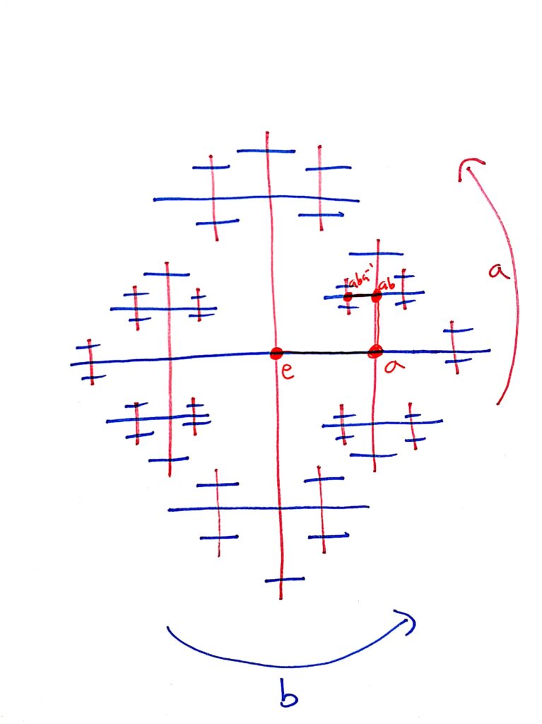
![\[aba^{-1} \cdot e = a \cdot (b \cdot (a^{-1} \cdot e)) = a \cdot (b \cdot a^{-1}) = a \cdot ba^{-1} = aba^{-1}\]](https://ggt.math.sites.carleton.edu/wp-content/ql-cache/quicklatex.com-a3946ae882c480956d7731dddc158b33_l3.png "Rendered by QuickLaTeX.com")
 , next to
  and finally to
  . To remind ourselves, I repeat the definition here.
 , and 3)
  on a hexagon. Indeed, fundamental domains are not unique, as we have seen from the very same example.
 such that condition 1) and 2) are satisfied. Then, we gradually shrink

 Define
  In other words, we would like to contain a minimal amount of vertices concerning how the group action can move things around.
 . Then, we want to show that every chain has a maximal element. We assume that we have the following chain:
 ranging over all
  in the chain. We claim that
 . Then, we assume that
  . There must exist
  such that
  . Thus, by assumption, we conclude that
  ; in other words, upon group actions,
 such that
  . Thus, since
  to any vertex in
  . Without loss of generality, we take the shortest path
  . Let
. Let  be the last vertex before arriving in
  is a larger set than
  such that
  , which is an exact rephrase of
  . Therefore, we have the desired contradiction.
 that is not covered in
  , should satisfy
  , where
  . Without loss of generality, we may append the half-edge containing
  for any
  , so we may as well consider the extension on
  , which we give the name
  , there exists
  .
. , where
  , note that
  .
. Then, by attaching half-edges, we obtain a star-like fundamental domain.
 Note that in the following picture, I draw the Cayley graph of
  generated by
  Here, I denote the black color as the edges corresponding to
  and the blue color as the edges corresponding to
  . Then, the two red highlighted portions denote two fundamental domains of
 , the stabilizer of
 , then those
  are exactly the stabilizer of the vertex
 and left cosets of
  given by
  Stab
Stab
 if and only if
  Thus, two elements in the orbit are the same if and only if their induced cosets are the same.
 where
where  is a fundamental domain for the action
  for one of the
  forms a transversal of
  .
. , a permutation of a graph which moves vertices to vertices and edges to edges in a one to one manner, while preserving the relationship between all aspects of a graph.
 has
has

 has labels and orientation.

 .
. .
. This direction requires us to show that
  so all we must do is verify that the action on edges, meaning that the action induces a map in
  . We define the action as
  , for
, for  , and
, and  . Now let’s take and edge
  and let
  act on both vertices. We obtain
  , so the action preserves the edge. Moreover, the result has the same label and orientation as
  where the label and orientation are all determined by the generating set
  For the other direction we must show that SYM
 SYM
SYM for
for  and
and  . The hypothesis will be that our map
  acts exactly the same as
  , defined as the unconnected neighborhood. Since each vertex in
  has exactly one adjacent edge along with a given label and orientation pair. By definition of SYM
 . It follows that
  .
. we have
  for some generating set
  . Finally, a more general statement about Cayley graphs is that we can read off relaters and equivalent words from that paths in a graph.
 such that
  .
.
 generates all of
  , and
, and  . Notice, since
  . As in the theorem conditions, we assume that
  for some
  which is valid since
  and
and  . We can thus in duct on this patter to find that
  for all
  and thus we can generate all of
![[G:H]=n](https://ggt.math.sites.carleton.edu/wp-content/ql-cache/quicklatex.com-2438bff8f10f99922f2baa1947f12f1f_l3.png "Rendered by QuickLaTeX.com") . □
. □![[G:H]](https://ggt.math.sites.carleton.edu/wp-content/ql-cache/quicklatex.com-b532b6cab9788a47c0ca03a4f9c1806c_l3.png "Rendered by QuickLaTeX.com") represents the degree of
represents the degree of  .
.
 such that
  and if
  then
then  .
. . For instance, the integers over addition can be conceived of as






 ?
? , does
  ?
?![\[g: X \to X, \text{ and } g: x \mapsto g \cdot x\]](https://ggt.math.sites.carleton.edu/wp-content/ql-cache/quicklatex.com-ea170b05f6d909c7a16dfc512c443ca6_l3.png "Rendered by QuickLaTeX.com")


![\[\varphi: G \to \text{Sym}X\]](https://ggt.math.sites.carleton.edu/wp-content/ql-cache/quicklatex.com-0aeac48530a3a607ff9e86b5a2a760d0_l3.png "Rendered by QuickLaTeX.com")
 is injective. Equivalently,
  such that
  , or in other words, that every non-identity element of
  . We define the action as
  . This action is faithful, because every non-identity
  . In other words, every configuration of
  as the multiplication operator of
  . This action will be associative because
  , and because
  , and let
  . We have that
  , so for every
  for some
  is injective. Thus
![\[G \cong \varphi(G)/\text{ker}\varphi \cong \varphi(G) \subseteq \text{Sym}X\]](https://ggt.math.sites.carleton.edu/wp-content/ql-cache/quicklatex.com-92d49d500bc8b4b3460c3fbcfe58b7f8_l3.png "Rendered by QuickLaTeX.com")
 , a multiset of edges
 and
and  are finite.
  is finite for all
  .
.  as the regular tree, given by a tree where every vertex connects to
  refers to a tree in which every vertex has either
  vertices.
  .
. ,
,  is disconnected.
  must be a bijective map of edges and vertices, and that
  is the graph of four points, each connected to every other point by an edge.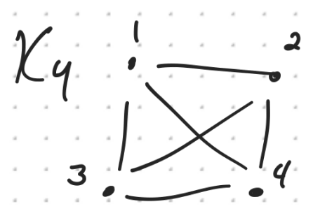
 , the symmetries on four elements.
 . It turns out that Sym
 , the rigid symmetries of a square.
 below mark where each part of its symmetry group come fromm and are not considered decorations:


 , as previously established, and Sym
 .
. such that
  for all
 such that

 . However, in this class we will generally use
  or
or 

 where each
  is called a relator. The set
  is also called the generating set.
 .
. and
and  . Relators can also show the relationship between two elements such that
  .
. since each of the other rotations is a power of
  since we can combine
  . By tradition we do not include
  and
and  as our set of relators. Therefore, our final group presentation is
  . Next time we will discuss how we know that this is enough to represent the entire group!
 .
.